Integrated Modeling Program and Total Cost of Ownership Calculator for Medium-Duty and Heavy-Duty Battery Electric Trucks in Regional Freight Use-Case Deployments PDF Free Download
1 / 51/51
100%

Integrated Modeling
Program and Total Cost
of Ownership Calculator
for Medium-Duty and
Heavy-Duty Battery
Electric Trucks in
Regional Freight Use-
Case Deployments
December
2024
A Research Report from the National Center
for Sustainable Transportation
Caleb Weed, Georgia Institute of Technology
Michael O. Rodgers, Georgia Institute of Technology and Oak
Ridge National Laboratory

TECHNICAL REPORT DOCUMENTATION PAGE
1. Report No.
NCST-GT-RR-24-45
2. Government Accession No.
N/A
3. Recipient’s Catalog No.
N/A
4. Title and Subtitle
Integrated Modeling Program and Total Cost of Ownership Calculator for
Medium-Duty and Heavy-Duty Battery Electric Trucks in Regional Freight
Use-Case Deployments
5. Report Date
December 2024
6. Performing Organization Code
N/A
7. Author(s)
Caleb C. Weed, https://orcid.org/0000-0002-7351-2416
Michael O. Rodgers, PhD, https://orcid.org/0000-0001-6608-9333
8. Performing Organization Report No.
N/A
9. Performing Organization Name and Address
Georgia Institute of Technology
School of Civil and Environmental Engineering
790 Atlantic Drive, Atlanta, GA 30332
10. Work Unit No.
N/A
11. Contract or Grant No.
USDOT Grants 69A3551747114, 69A355122344814
Ray C Anderson/Drawdown Georgia Grant
12. Sponsoring Agency Name and Address
U.S. Department of Transportation
Office of the Assistant Secretary for Research and Technology
1200 New Jersey Avenue, SE, Washington, DC 20590
Ray C. Anderson Foundation
1180 West Peachtree Street NW, Suite 1975, Atlanta, GA 30309
13. Type of Report and Period Covered
Final Research Report (February 2021 – June 2024)
14. Sponsoring Agency Code
USDOT OST-R
15. Supplementary Notes
DOI: https://doi.org/10.7922/G2R20ZQT
Total Cost of Ownership Spreadsheet Tool: https://doi.org/10.5281/zenodo.14589111
16. Abstract
This report outlines the technical development and application of the Total Cost of Ownership Spreadsheet Tool (TCOST), a
Microsoft Excel-based calculator that simplifies and integrates the main functions, data, and outputs of pre-existing models
(MOVES-Matrix and the GREET Model) and other external sources of economic data. The tool accommodates twenty-one user-
input variables to produce comparative total cost of ownership figures for diesel and battery-electric trucks within any use case,
broken down by cost type (capital, operation, and maintenance), both as a gross number and on a per-mile basis. The tool also
provides a series of visualizations comparing cost breakdowns, breakeven points, and expected tailpipe and fuel-cycle emissions
for both technologies. A hypothetical regional container drayage use-case example was developed using quantitative and
qualitative data, to which TCOST was applied to demonstrate the application of the tool and its value to fleet managers and
policymakers in its ability to model the cost effects of minor parameter adjustments or the multiplicative effects of simultaneous
parameter adjustments quickly and easily. TCOST may be used to help inform the decision-making process for fleet vehicle
acquisition and planning, helping decision makers to visualize a variety of future scenarios and map those scenarios onto their
fleet operations to assess risks and make informed choices about the future technological makeup of their fleets. TCOST will help
policymakers quickly model the cost impacts of potential policy levers from a business perspective.
17. Key Words
Electric Vehicles, Trucks, Freight, Electrification, Energy, Emissions, CO2
18. Distribution Statement
No restrictions.
19. Security Classif. (of this report)
Unclassified
20. Security Classif. (of this page)
Unclassified
21. No. of Pages
51
22. Price
N/A
Form DOT F 1700.7 (8-72)
Reproduction of completed page authorized

About the National Center for Sustainable Transportation
The National Center for Sustainable Transportation is a consortium of leading universities
committed to advancing an environmentally sustainable transportation system through cutting-
edge research, direct policy engagement, and education of our future leaders. Consortium
members include: the University of California, Davis; California State University, Long Beach;
Georgia Institute of Technology; Texas Southern University; the University of California,
Riverside; the University of Southern California; and the University of Vermont. More
information can be found at: ncst.ucdavis.edu.
Disclaimer
The contents of this report reflect the views of the authors, who are responsible for the facts
and the accuracy of the information presented herein. This document is disseminated in the
interest of information exchange. The report is funded, partially or entirely, by a grant from the
U.S. Department of Transportation’s University Transportation Centers Program. However, the
U.S. Government assumes no liability for the contents or use thereof.
The U.S. Department of Transportation requires that all University Transportation Center
reports be published publicly. To fulfill this requirement, the National Center for Sustainable
Transportation publishes reports on the University of California open access publication
repository, eScholarship. The authors may copyright any books, publications, or other
copyrightable materials developed in the course of, or under, or as a result of the funding grant;
however, the U.S. Department of Transportation reserves a royalty-free, nonexclusive and
irrevocable license to reproduce, publish, or otherwise use and to authorize others to use the
work for government purposes.
Acknowledgments
This study was funded, partially or entirely, by a grant from the National Center for Sustainable
Transportation (NCST), supported by the U.S. Department of Transportation (USDOT) through
the University Transportation Centers program. The authors would like to thank the NCST and
the USDOT for their support of university-based research in transportation, and especially for
the funding provided in support of this project.

Integrated Modeling Program and Total
Cost of Ownership Calculator for Medium-
Duty and Heavy-Duty Battery Electric
Trucks in Regional Freight Use-Case
Deployments
A National Center for Sustainable Transportation Research Report
December 2024
Caleb Weed, Civil and Environmental Engineering, Georgia Institute of Technology
Michael O. Rodgers, Ph.D., Civil and Environmental Engineering, Georgia Institute of Technology, and
National Transportation Research Center, Energy Science and Technology Directorate,
Oak Ridge National Laboratory

[page intentionally left blank]
i
TABLE OF CONTENTS
EXECUTIVE SUMMARY .................................................................................................................... iv
Introduction .................................................................................................................................... 1
Truck Freight Use-Case Study within Georgia’s Freight System ..................................................... 4
Use-Case Selection ...................................................................................................................... 9
Total Cost of Ownership Spreadsheet Tool .................................................................................. 25
TCOST Application in the Use-Case Example ............................................................................ 28
Conclusion ..................................................................................................................................... 33
References .................................................................................................................................... 34
Data Summary............................................................................................................................... 39
Appendix A: TCOST Emissions Rates ............................................................................................. 40
Appendix B: Use-Case Example Inputs to TCOST.......................................................................... 41
ii
List of Tables
Table 1. BE truck sales percentage schedule (CA Code of Regulations 1963-1963.5) [10] ............ 2
Table 2. Route segment attributes ............................................................................................... 13
Table 3. MOVES-Matrix default inputs (SourceType 62, MY2008)............................................... 15
Table 4. OpMode bin definitions in MOVES ................................................................................. 17
Table 5. Use-case on-road emissions rates (grams per mile) in 2022 .......................................... 18
Table 6. Financial parameters ....................................................................................................... 21
Table 7. Total cost of ownership breakdown (with charging systems) ........................................ 22
Table 8. Upstream emissions from fuel cycle from GREET ........................................................... 23
Table 9. TCOST default vehicle parameters .................................................................................. 27
Table 10. Well-to-pump ................................................................................................................ 40
Table 11. Pump-to-wheels ............................................................................................................ 40
Table 12. Use-Case Example Inputs to TCOST .............................................................................. 41
iii
List of Figures
Figure 1. Significant freight corridors in Georgia [19] .................................................................... 6
Figure 2. Truck volumes in the Atlanta region [20] ........................................................................ 7
Figure 3. Total freight moved by distance in 2022 [28] ................................................................ 10
Figure 4. Appalachian Regional Port facility [30] .......................................................................... 11
Figure 5. ARP to distribution center drayage use-case route [33] ............................................... 12
Figure 6. Composite driving cycle profile for ARP drayage use-case............................................ 15
Figure 7. Heavy truck gross weight distribution [40] .................................................................... 16
Figure 8. Distribution center drayage OpMode bin distribution .................................................. 18
Figure 9. Predicted diesel price through 2040 [53]. ..................................................................... 20
Figure 10. Predicted commercial electricity rates through 2040 [53]. ......................................... 20
Figure 11. Vehicle energy efficiency ratio by average speed from CARB [54] ............................. 22
Figure 12. Total ICE lifetime emissions (kgs) ................................................................................ 23
Figure 13. Total BEV lifetime emissions (kg) ................................................................................. 24
Figure 14. TCOST input cells.......................................................................................................... 26
Figure 15. Diesel truck schedule of costs from TCOST ................................................................. 29
Figure 16. BE truck schedule of costs from TCOST ....................................................................... 30
Figure 17. TCO comparison from TCOST....................................................................................... 30
Figure 18. Emissions comparison from TCOST ............................................................................. 31
Figure 19. Sensitivities of selected input parameters in use-case example ................................. 32
iv
Integrated Modeling Program and Total Cost of
Ownership Calculator for Medium-Duty and Heavy-Duty
Battery Electric Trucks in Regional Freight Use-Case
Deployments
EXECUTIVE SUMMARY
Over the past decade, battery-electric vehicle (BEV) technologies have made tremendous
strides in technical performance and cost-effectiveness, compared to conventional combustion
engines. The ability of BEVs to reduce emissions and operating costs has catapulted the
technology to the forefront of conversations within sustainable transportation, especially with
increasing downward pressure by an evolving policy landscape on fleet operators and original
equipment manufacturers (OEMs) to reduce the on-road environmental footprint of their
vehicles. So far, the vast majority of successful BEV deployments have occurred in light-duty
market segments, but heavier vehicle classes are beginning to receive more attention for their
electrification prospects.
Medium- and heavy-duty vehicles (MHDVs) represent significant opportunities for the
deployment of BEV technologies. While some success has been achieved in electrifying transit
buses, the vast majority of MHDV on-road activity is in freight transportation. Freight trucks are
responsible for nearly 25% of emissions from the U.S. transportation system, or about 7% of
national greenhouse gas (GHG) emissions. In addition to GHG emissions, diesel truck activity is
currently a major source of criteria pollutant emissions, including fine particulate matter and
oxides of nitrogen, which can be detrimental to human health and the environment. OEMs
have identified MHDVs in freight applications as a potential market for BEV technology and
have begun to advertise electric MHDVs to fleet operators as opportunities to reduce operating
and maintenance costs. However, the benefits of electrification can be highly nuanced and may
vary substantially depending on complex interactions between vehicle activity, duty cycle,
payload, and the physical environment, including road topography and meteorology, as well as
characteristics from the electrical power grid used to charge battery electric vehicles.
A central issue for BEV deployment in the freight sector is advancing the understanding of the
specific vehicle use-cases and operational conditions for which electrification is a viable
solution. Identifying the business activities and business economic environment, coupled with
on-road operating activity conditions in which BEVs can successfully replace conventional
vehicles, is complicated. However, achieving the highest impact reductions in emissions and
reduced operating expenses is critical to ensuring that the most effective deployments of
battery vehicle technology are implemented. This report outlines methods that can be used to
quantify the lifecycle energy use, emissions, and economic implications of targeted
deployments of electric trucks within freight use cases and optimal operating conditions for
electrification. This report will demonstrate the quantification process for a hypothetical
regional container drayage use-case example.
v
To aid in investigations of this nature, the research presented in this report outlines the
technical development, and intended applications of a new tool dubbed the Total Cost of
Ownership Spreadsheet Calculator (TCOST). The new TCOST model integrates a set of simplified
functions with energy use and emission rate outputs from a group of preexisting models to
produce comparative lifecycle emissions, energy consumption, and total cost of ownership
figures for battery-electric and conventional diesel trucks performing the same on-road activity.
The tool is intended to facilitate expedited and simplified inquiries into the technical and cost
comparison between conventional trucks and comparable BEVs, to identify use-cases and
conditions that should be prioritized for electrification so that ongoing electrification
investment will maximize economic and environmental benefits over time. The tool’s broad
applicability, facilitated by its simple interface and customizable user-inputs that support the
assessment of a vast array of possible modeling scenarios, will be of great value to a diverse
range of fleet operators and policymakers, because the model provides a simple method for
gaining quick insights into the economic and environmental implications of fleet management
and regulatory decisions.
1
Introduction
The Intergovernmental Panel on Climate Change (IPCC) concluded that only rapid, deep
decarbonization, and implementation of climate change mitigation actions by the end of this
decade can reduce disruptive and costly damage to human and natural systems [1]. Given the
high risk of deleterious consequences of delayed implementation of greenhouse gas (GHG)
abatement programs, given that transportation is the highest-emitting economic sector in the
United States (responsible for more than 25% of total GHG emissions), and given the criticality
of road transportation subsystems to higher order social and economic systems, the IPCC places
great emphasis upon the accelerated maturation of alternative transportation fuels, low-
emissions vehicle technologies, and reconfigured operational designs to pursue reduced energy
consumption and GHG abatement. In recent years, accelerated rates of innovation have made
alternative powertrains (parallel hybrid, plug-in hybrid (PHEV), battery-electric (BE)), and fuels
(electricity, compressed/liquified natural gas (C/LNG), hydrogen (H2)) much more competitive
with traditional fossil fuel powered internal combustion engine (ICE) powertrains in the light-
duty vehicle (LDV) market. LDV BEVs have made especially large strides in technological
maturation, supported by multilateral policy encouraging research, development, adoption,
and charging infrastructure network improvements.
While electrification prospects for LDVs are well established, those for medium- and heavy-duty
vehicles (MHDVs) are less clear. MHDVs are essential to nearly all sectors of the economy and
represent significant opportunities for BE technology deployments. In 2019, nearly 12 billion
tons of freight were moved by MHD trucks, representing nearly 64% of national freight tonnage
and value. Tonnage is expected to grow by about 1.4% per year until at least 2050 [2].
Additionally, 25% of fossil fuel consumption and GHG emissions from transportation in the
United States come from MHDVs [3]. Because a typical MHDV consumes much more fuel than a
LDV, each electric MHDV can yield greater environmental benefits than a single electric LDV.
The scale and importance of trucks to the global economy and their corresponding energy
consumption has given rise to a growing catalogue of BE MHDV models on the market for
freight applications [4]. Original equipment manufacturers (OEMs) have identified an emerging
market for BE MHDVs, advertising them to fleet operators as an opportunity to reduce
operating and maintenance (OM) costs and their ecological footprint. While environmental
benefits of BEVs are broadly appreciated, they can vary substantially depending on complex
interactions between vehicle behavior (such as on-road driving cycle and payload), the physical
environment (such as topography and meteorology), as well as characteristics of the electrical
power grid used to charge these vehicles [5].
Due to the nuanced complexities of freight truck electrification, the MHDV market has focused
BEV deployment strategies to target specific vocations that have operational characteristics
that are the most conducive to electrification. Local small parcel delivery vehicles have received
the most attention, due to the relatively low daily miles travelled (i.e., within the range of a
single battery pack charge) and lower loads and less strenuous duty-cycles that do not require
larger battery capacity. Signaling the attractiveness of BEV deployments in parcel delivery
vocations, the United States Postal Service (USPS) awarded contracts for over nine thousand

2
BEVs and over fourteen thousand charging stations in early 2023 in support of the agency’s
stated goal to make 75% of its newly acquired vehicles electric, rising to 100% in 2026 and
thereafter [6]. The United Parcel Service (UPS) has a similar goal of reaching 40% alternative
fuel in the company’s ground operations by 2025 and carbon neutrality by 2050. UPS currently
boasts over one thousand BEVs and PHEVs on the road in support of that goal and has
agreements in place to purchase thousands more [7]. Other vocations have also begun to reap
the benefits of BE MHDVs in recent months as well. In late 2022, PepsiCo received the first
order of Class 8 Tesla Semi electric trucks for deployment in their beverage delivery operation.
Frito-Lay, a PepsiCo subsidiary, deployed 40 electric vans within their North American division
last year [8]. PepsiCo’s Class 8 heavy-duty trucks will operate on short and regional haul duty
cycles. While the electrification of long-haul heavy-duty semitrucks has been studied closely,
the significantly greater trip lengths, payloads, and subsequent greater energy demands and
fuel consumption, necessitate larger and more powerful batteries for HDV electric powertrains
than are provided by current technology in most cases. BEV models capable of long-haul
operations are on the horizon, but existing BE MHDVs have operational ranges of less than 250
miles, with a few but growing number of exceptions [9].
Policy levers orchestrated by local, state, and national governments have also helped to
accelerate much of the recent growth observed in truck freight electrification. In 2021, the
California Air Resources Board (CARB) finalized their Advanced Clean Trucks rule, setting a
standard requirement for 50% of new medium- and light heavy-duty vehicle (Class 4-6) and 30%
of new heavy-duty tractor (Class 7-8) sales to be zero-emitting by 2030 as shown in Table 1 [10].
CARB is currently taking public comments on an updated clean trucks plan that is even more
ambitious [11]. New York state adopted a similar rule, establishing a ratcheting standard for
percentage of new electric MHDV sales as a share of total MHDV sales, culminating in 100% of
new MHDVs registered in the state being zero-emitting by 2045 [12]. In addition, a coalition of
17 US states plus Washington D.C. and the province of Quebec, Canada signed a memorandum
of understanding in 2022 committing to reaching 30% of new MHDV sales being zero-emitting
by 2030, rising to 100% by 2050 [13]. This coalition estimates the potential net economic
savings of the full electrification of the national MHDV fleet to be as much as $140 billion
cumulatively, across the vehicles’ lifetimes [14].
Table 1. BE truck sales percentage schedule (CA Code of Regulations 1963-1963.5) [10]
Model Year
Class 4-6
Class 7-8
2025
11%
7%
2030
50%
30%
2035 and beyond
75%
40%
At the Federal level, the United States Environmental Protection Agency (U.S. EPA) announced
a proposed rule that applies more ambitious pollution standards to heavy-duty vocational
vehicles, and CARB projects that the new rule will avoid 1.8 billion metric tons of GHG emissions
3
between 2027 (the first model year subject to the rule) and 2055, and provide significant
particulate matter and other criteria pollutant emission reductions. According to the U.S. EPA,
the industry can meet the new standards by achieving 50% zero-emissions vehicles for
vocational vehicles, 34% for day use tractors, and 25% for sleeper cab tractors in MY2032, with
a mix of BE and fuel cell technologies. The U.S. EPA also projects significant savings for electric
MHDV purchasers due to reduced operating costs, despite increased upfront costs and after
accounting for available battery tax credits [15].
The regulatory focus on, and the consideration afforded to, electric trucks in present and future
plans of players in the road freight industry signal an emerging alignment on the public and
business benefits of electric MHDVs. There is widespread agreement in the freight industry that
electrification can be a sound business choice, with operating mode savings surpassing higher
MSRPs relatively early in the ZEV’s useful lifetime. In support of their rulemaking, the U.S. EPA
found that most zero-emitting MHDV purchasers would offset their increased upfront costs,
including the cost of electric vehicle supplementary equipment (EVSE) like charging
infrastructure, with operational savings within three years of ownership [15]. Elsewhere, Gao et
al (2017) simulated energy consumption of a Class 7 local food delivery truck and found a
battery electric or Power-GenSet PHEV (Power-GenSet implying the vehicle’s downsized
combustion engine is used only to generate electricity to recharge the PHEV battery when
needed) can reduce the overall cost for energy by 29 to 44 percent, with the noted variability
attributable to on-route charging availability, payload characteristics, and other factors [16].
However, these authors did not consider the increased cost of electric powertrain technology.
Another study assumed a MSRP differential of around $100,000 between a conventional Class 8
diesel and battery-electric semi-truck and found a baseline payback period for the BEV of 3.24
years ±1.46 years [17].
The reality remains, however, that the magnitude of savings and payback periods are heavily
dependent upon each vehicle’s routes, on-road operating characteristics, and the design of the
freight distribution system for each electrification application. A primary analytical goal of fleet
electrification assessment is to identify what makes one use-case more attractive for BE
technology deployment than another. This requires knowledge of the operational
configurations of the fleet and availability of an analytical tool that can assess electrification
benefits. A simple, standardized technoeconomic analytical framework can leverage preexisting
economic and lifecycle models, while also reducing the modeling knowledge required to
evaluate the electrification merits for specific conditions. The TCOST model is designed to help
identify feasible use cases that can lead to the most efficient rollout of electrification within
specific sectors/businesses in the MHDV fleet. The TCOST model implements an economic
analysis framework that can be applied to any freight sectors wherein fleet composition, freight
loads, and on-road activity can be quantified, and then calculates economic benefits and
disbenefits of BEV deployment, as well as energy use and emission reduction benefits by
applying existing energy use and air quality models (the U.S. Environmental Protection Agency’s
MOVES model, implemented in a matrix form known as MOVES-Matrix, and the U.S.
Department of Energy’s GREET model) within the economic analysis framework. As part of this
research, an example short-range to-mid-range MHDV freight use-case is assessed using TCOST

4
for the state of Georgia. The use-case example operating profiles presented in this report
indicate how specific drayage freight flows can bring into focus the characteristics that help or
hinder electrification potential.
The Total Cost of Ownership Spreadsheet Tool (TCOST) is provided as a Microsoft Excel®-based
model (https://doi.org/10.5281/zenodo.14589111), distilling the framework utilized in the use-
case evaluation down to a simple user interface with a series of inputs to customize calculations
for user-defined use-cases. TCOST integrates primary data, functions, and assumptions of
MOVES-Matrix for “Pump-to-Wheels” (PTW) energy consumption and emissions rates, and the
DOE GREET model (for fuel pathway mixes and upstream “Well-to-Pump” (WTP) energy
consumption) while also incorporating from the literature, additional information relevant to
the simulations. TCOST expedites the analytical process and vastly reduces required modeling
knowledge for MHDV electrification analyses, removing knowledge barriers and facilitating
more efficient and effective decision-making for freight brokers and MHDV fleet managers.
Finally, TCOST is applied to the previously defined use-case to demonstrate its utility for fleet
managers and planners as a simplified method for back-of-envelope calculations using a
handful of user inputs to assess benefits and inform decision-making. The TCOST application to
the use-case serves as an instructional model for future use of the tool.
Truck Freight Use-Case Study within Georgia’s Freight System
Understanding the form, trends, and operational conditions of Georgia’s freight system is
important because it provides a context against which individual vocations can be evaluated.
Handling over 850 million tons of freight flows annually, the state of Georgia boasts one of the
most robust freight networks in the United States. The state is home to the nation’s most
significant airport for air cargo with Hartfield-Jackson International (HJIA), the fastest growing
container port with the Port of Savannah (POS), and the southeast hub of operations for two
Class I railroads in the eastern U.S. with Norfolk Southern (NS) and CSX. Georgia’s Interstate
system is in the top ten among states for interstate miles (1,243 miles), and Georgia has an
extensive network of state highways and local roads providing enhanced connectivity. The
state’s logistic industry is a critical component of the state economy; in 2018 logistics was
responsible for about 7% of Georgia’s GDP ($46.6 billion) and nearly 500 thousand jobs,
including 239 thousand direct jobs [18].
In Georgia, 75% of total 2018 freight flows by weight (excluding the pipeline mode) are carried
by truck, with almost the entire remaining 25% of total tonnage carried by rail. An even larger
share of freight value (about 88%) was carried by truck [18]. Truck freight is uniquely positioned
to provide door-to-door service between almost any origin and destination, enabling highly
flexible delivery scheduling at low cost and on short notice. For this reason, truck mode share
and total volume in Georgia are forecasted to grow substantially, in line with the growth of
same-day or next-day deliveries associated with e-commerce. Truck freight flows in Georgia are
expected to grow anywhere from 1.5% per year (TRANSEARCH estimates) to 2.2% per year
(American Trucking Association (ATA) and Economy.com estimates) through mid-century [19].
5
Georgia’s truck freight system activity is geospatially centered around the Metro Atlanta region
as well as the Port of Savannah. Atlanta is the second largest population center in the southeast
U.S. and is a major manufacturing and commercial hub. The Port of Savannah is the second
busiest container port in terms of total throughput on the East Coast [20]. Figure 1 shows the
convergence of multiple significant freight corridors in Georgia’s Atlanta region for both
interstate (within state) and intrastate (between state) commodity flows. Figure 2 is from the
Atlanta Regional Commission’s (ARC) latest regional freight mobility plan published in 2016 and
depicts truck volumes on the Interstate system and state highways in the Atlanta region. The
dense truck traffic on the I-285 perimeter is primarily due to interactions between through
truck movements generated outside of the metro area with destinations also outside of the
region (trucks may not enter the I-285 Perimeter without a permit to pick-up or drop-off
freight), coupled with local delivery trucks transporting goods between warehouses and
distribution centers and to locations within the region. The top twelve truck count locations in
Georgia are in the Atlanta metropolitan region [19]. The restriction of activities on I-75 and I-85
inside the I-285 perimeter lead to comparatively low truck counts on those thoroughfares.
The Atlanta-Savannah corridor is especially significant to the economic wellbeing of Georgia as
it connects the state’s regional economic and population center with the Southeast’s primary
link to the international market at the Port of Savannah. Over 100 thousand loaded trucks
complete trips between Atlanta and Savannah every year (averaging more than 400 trucks per
day, assuming 250 workdays in a year), and three intermodal trains also depart every day [20].
These numbers have only grown since the Georgia Ports Authority completed a deepening
project in Savannah harbor in 2022, which is estimated to allow a typical container ship to load
an additional one thousand containers and increase import and export volumes at the Port of
Savannah [21].

6
Figure 1. Significant freight corridors in Georgia [19]

7
Figure 2. Truck volumes in the Atlanta region [20]
The growth of the Port of Savannah has been accommodated by the maturation of intermodal
drayage systems that provide more efficient container freight flows via inland ports in central
Georgia, the Atlanta region, and beyond. For example, the Cordele Intermodal Facility (CIF) in
Cordele, GA, is a prominent private truck-rail intermodal transfer facility located south of
Macon, GA that boasts direct railroad service to the Port of Savannah. Incoming and outgoing
containers can be moved by freight rail between CIF and Port of Savannah, being loaded and
offloaded onto trucks further inland at CIF [22]. The inland, central location of CIF shortens the
distance of required truck trips rather than relying entirely on direct truck service to POS; CIF is
64 miles from Macon, 147 miles from the Norfolk Southern Inman Yards intermodal complex in
the Atlanta area, 121 miles from Tallahassee, Florida, and within much shorter distances to
agricultural production centers in south-middle Georgia. Trucks need to travel less than two
miles from CIF for I-75 access.
8
The Georgia Ports Authority (GPA) owns and operates inland ports of their own. Appalachian
Regional Port (ARP) in northwest Georgia is operated in public-private partnership with CSX.
ARP has direct CSX railway connection to the Port of Savannah and easy access to the I-75
corridor, providing inland intermodal transfers about 100 miles from both Atlanta and
Knoxville, TN and 45 miles from Chattanooga, TN. GPA benchmarked the capacity of ARP at 50
thousand containers per year when it opened in 2018 and there are plans to double its capacity
by 2028 [23]. GPA estimates each round-trip container moved by rail to and from ARP to offset
710 truck miles on Georgia’s highways and the port diverts up to 40 thousand trucks from
Atlanta area roadways each year [18, 24]. Bainbridge Terminal in southwest Georgia primarily
handles intermodal transfers for containers traveling by barge on the Apalachicola-
Chattahoochee-Flint waterway system in that part of the state. Construction plans for another
inland port facility in Hall County, northeast of the Atlanta region, gained federal environmental
approval in May 2023. GPA estimates construction to be completed in 2026 [25]. There are also
five additional intermodal rail terminals located in the Atlanta region [20].
Expansion of intermodal and inland port capabilities can significantly lower transportation costs
for commodity import and export flows, helping to make global markets more cost-
competitive, accelerating regional economic development, and attracting business. By
extending the gates of container ports inland, inland port systems enable shippers to efficiently
serve new logistics pathways supporting online business divisions and e-commerce. Being able
to serve customers with next-day, same-day, or even one-hour parcel deliveries is highly
valuable to businesses, and many have reorganized their supply chains into multichannel
configurations by replacing regional distribution centers with smaller, forward distribution
centers in urban areas. Many of these warehouses need to be replenished with multiple
incoming truckloads each day, in addition to generating many outgoing trips for local deliveries.
Such fulfillment centers are increasingly co-located with manufacturing centers and intermodal
ports, leading to more numerous and larger freight clusters around intermodal rail heads [20].
Three commodities, “mixed freight,” “plastics and rubber,” and “other foodstuffs,” appear in
the top ten commodities in Georgia for both ton-miles and value [26]. Mixed freight is a
commodity group suggesting the cargo consists of a variety of different types of products. It is
the most common commodity arriving at distribution centers as well as many retail businesses
and restaurants because the commodity can include certain food items, hardware, office
supplies, clothing, and much more [27]. Because distribution centers often handle a variety of
goods to serve their customers, the generalized nature of the mixed freight commodity make it
a useful classification and reduce administrative burden, compared with using multiple specific
product classifications. While not all mixed freight movements can be unequivocally associated
with distribution centers, freight flows for the commodity are more likely to be observed along
intermodal freight systems in drayage movements between intermodal terminals and
fulfillment centers, and beyond in delivery movements to customers and points of sale.
Because of its expected on-road behavior, the commodity is more likely to be one that could
technically achieve high penetration of BE truck technology.
9
The frequent proximity of forward distribution centers, intermodal ports, and population
centers improve electrification prospects for vehicles on freight vocations connecting these
locations by shortening typical trip distances and encouraging a “out-and-back” tour cycle,
where trucks begin and end their routes at the same location, making charging equipment
siting more straightforward. It is hypothesized that trips to and from intermodal ports could
have a relatively high number of operational characteristics that make these flows high value
opportunities for investment in BE deployments, especially as intermodal flows continue to
grow. High utilization and miles traveled typically improve the economics of BEVs. Increasing
trip frequencies could represent increasing electrification benefits, so long as BE technology can
adequately fulfill service demands within the constraints of battery capacity and charging
requirements. Exploring these parametric relationships and testing these hypotheses was
central in the design of the use-case study.
Use-Case Selection
In the developing a use-case profile, national truck freight trends were first examined, to help
inform assumptions about truck activity in Georgia where data gaps exist. National freight
statistics provide a more comprehensive understanding of the broader freight system and
trends, which can be scaled down to state-level systems. Many currently observed trends in the
United States freight network have energy use implications that are important to consider as
technical and economic electrification feasibility is studied. Doing so provides critical context
for the activity of any specific use-case and helps to enable transferability of findings of
electrification analyses such as these. That is, understanding overall trends makes it easier to
identify patterns as well as outliers of system form and function that positively or negatively
affect electrification potential, making identification of ideal use-cases simpler. This study
considers several national truck freight trends that have a direct influence on use-case energy
consumption and technoeconomic feasibility of BEV technology deployments:
• In 2022, 73.8% of weight and 55.5% of value of goods traveling by truck mode moved
less than 250 miles between origin and destination, as depicted in Figure 3 [28]. Most of
these freight flows, assuming payloads and driving conditions are reasonable, fall within
the technically achievable operational range of current BE technologies.
• About 95.7% of MHDV fleets consist of ten or fewer trucks, and 99.7% of MHDV fleets
operate with fewer than one hundred units [29]. Operational data for private fleets is
not accessible to the public. However, understanding the typical fleet size is important
for assessing the benefits of any economies of scale that arise from investing in multiple
BEVs at once, such as those from charging equipment investments. It is also valuable for
benchmarking charging demand and modeling different fleet charging schedules.

10
Figure 3. Total freight moved by distance in 2022 [28]
Keeping these national observations in mind, a MHDV use-case in Georgia was identified for
further electrification analysis. Given the lack of access to proprietary operational data for
private fleets, the use-case is largely reconstructed using assumptions to fill data gaps to create
realistic hypotheticals. Relevant operational characteristics and model inputs cannot be known
without private industry participation, so the analysis is supplemented by robust sensitivity
analysis to evaluate a range of possible iterations of the same overall freight movement. For a
fleet manager performing such an analysis, much of the missing data would be known and the
analysis could be similarly executed but with much greater precision.
Appalachian Regional Port Drayage
The use-case designed for further analysis is a hypothetical mixed-freight drayage operation
from ARP to a distribution center in Adairsville, Georgia, northwest of the Atlanta metropolitan
area. ARP is in Murray County in central north Georgia and serves as an intermodal transfer
facility, switching containers between rail and heavy truck. The facility is directly serviced by
CSX, which offers rail service on a direct route of 388 miles to the Port of Savannah Garden City
Terminal. Its capacity is over 50 thousand containers per year, and it is on target to grow to
handle 100 thousand containers per year by the end of the decade [23]. The plans for the
facility are shown in Figure 4.
36.0% 37.4%
12.8%
3.8% 3.3% 4.1% 1.3% 1.3%
36.0%
73.4%
86.2% 90.0% 93.3% 97.4% 98.7% 100.0%
Below 100 100 - 240 250 - 499 500 - 749 750 - 999 1,000 -
1,499
1,500 -
2,000
Over 2,000
Cumulative Percent
Percent of Total
O-D Distance (miles)

11
Figure 4. Appalachian Regional Port facility [30]
The distribution center is modeled on the 1.4 million square foot distribution center for a major
hardware retailer that exists on the location [31]. This terminus is 61.1 miles from ARP using a
truck-friendly route [32]. Figure 5 shows the route in Google Maps and Table 2 breaks each leg
of the route into segments and portrays some of their roadway characteristics.

12
Figure 5. ARP to distribution center drayage use-case route [33]
Note: The discrepancy between the Google Maps portrayed distance and the actual on-road distance is due to a
Google Maps routing error misprocessing the outbound alignment of the ARP to be right-turn only. The actual
distance is 61.1 miles.

13
Table 2. Route segment attributes
No.
Road
Segment
Length
(miles)
Speed
Limit
(mph)
Road
Class
Notes
1
US 411/GA
2/ GA 61
8.0
35/45
Major
collector
2 lanes at ARP, growing
to 4 on southbound
approach to Eton, GA
2
US 76/GA
52
8.3
45
Principal
Arterial
4 lanes
3
US 41/US
76/GA 3
6.1
45
Principal
Arterial
4 lanes
4
I-75
30.2
70
Interstate
6 lanes
5
GA 140
7.6
50
Minor
Arterial
4 lanes through
Adairsville, 2 lanes from
Adairsville to end of
segment. Construction is
ongoing to make 4 lanes
for the entire segment.
6
Prosperity
Way
0.3
Not posted
Local
Road
2 lane access road.
Distribution center is
only business on
alignment.
Container drayage is typically conducted using Class 8 combination tractor trailer day cab units.
For this use-case, we assume that the fleet is a small privately owned and operated third-party
logistics (3PL) operation consisting of three MY 2008 Class 8 combination trucks, all performing
similar drive cycles on the same route. The trucks are assumed to travel from ARP to the
distribution center with a full 20-foot shipping container of payload. Upon arrival, the full
container is unloaded on-chassis at a staging area or delivery bay. The truck then picks up an
empty container chassis and returns to ARP. The total distance of the tour on public roads (i.e.,
from gate to gate) is 122.2 miles. The vehicles have been operating on this vocation since their
acquisition. The owner-operator is planning to evolve their fleet and is seeking to understand
how the energy use and economic implications of fleet management decisions will affect their
business. They have decided to replace their vehicles with new MY 2023 trucks and want to
understand electrification potential for their operation. To quantify the pros and cons of fleet
electrification compared to the purchase of new traditional diesel trucks, we analyze both on-
road and upstream energy consumption and emissions for each technology and fuel type for
this use-case. We also quantify fuel, maintenance, and capital costs of both purchasing
scenarios.
MOVES is the federal regulatory model for quantifying on-road emissions and energy
consumption for any use-case. MOVES essentially calculates the second-by-second power
demand (kilowatts per metric ton) for a vehicle in units of vehicle specific power (VSP), or in the

14
case of heavy-duty vehicles, scaled tractive power (STP). STP is essentially equivalent to VSP,
except that STP integrates a large fixed mass factor to account for medium-duty and heavy-duty
vehicle payload. VSP and STP are functions of vehicle speed, acceleration, and mass (see
Equation 1):
(1)
VPS is calculated at 1-hz resolution, where A is rolling resistance in kW-sec/meter, B is rotating
resistance in kW-sec2/m2, C is aerodynamic drag in kW-sec3/m3, vt is velocity in m/sec at time t,
at is acceleration in m/sec2 at time t, g is gravitational acceleration (9.81 m/sec2), θt is road
grade in degrees, m is vehicle mass in metric tons, and M is a scaling factor to relate VSP and
STP ranges [35].
For this analysis, road grade impacts on energy consumption are not considered. This area of
northern Georgia does possess considerable elevation changes and the presence of grade on
truck routes could significantly improve or hinder electrification process. Route segments with
high percentages of downgrade are opportunities for energy savings and charge regeneration
via regenerative braking systems. Routes with steep upslopes increase energy demand on the
driving cycle. Given that downgrades never recover all of the energy lost moving uphill, routes
with significant grace can limit the feasibility of some routes for BE MHDV applications. Grade
effects impact outcomes on a case-by-case basis and warrant inclusion in subsequent studies
but are out of scope here. In the TCOST tool, which will be discussed in the next section, energy
demand effects of road grade are captured by the fuel consumption user input which informs
the model’s energy use assumptions.
To calculate VSP for every second of the vehicle’s driving cycle, a driving cycle with 1-hz speed
and acceleration data is required. To capture the energy consumption effects of evolving driver
behavior across different road types on this tour, a composite driving cycle was created using
various standard regulatory cycles for heavy duty trucks with some modifications. In this
manner, the generated driving cycle was crafted to be as realistic as possible until telematic
device deployment can provide second-by-second data. The driving cycle is one-way between
ARP and the distribution center. Its profile is depicted in Figure 6, which is color-coded to show
how each segment of the trip was combined. The composite driving cycle was manufactured
using various heavy heavy-duty truck cycles made available by Georgia Tech through the U.S.
EPA and state regulatory agencies. The beginning of Segment 5, which is the leg of the trip on
GA 140 between the I-75 exit ramp and the distribution center access road (Prosperity Way), is
a modified version of a U.S. EPA HHD truck creep cycle used for characterization for truck
emissions in California [36]. The total travel time for this one-way driving cycle is 104.3 minutes.
For simplification, we assumed a truck on this use-case would execute this driving cycle with a
full container load before executing it again in reverse with an empty container as the return
trip.

15
Figure 6. Composite driving cycle profile for ARP drayage use-case
MOVES-Matrix was developed at Georgia Tech to drastically reduce calculation times for
MOVES runes by pre-processing hundreds of thousands of unique combinations of input
variables and capturing outputs for lookup in a multidimensional array [37]. Here, the default
physics parameters for a MY 2008 and a MY 2023 Class 8 combination long-haul truck
(SourceTypeID 62 in MOVES-Matrix) were used for energy consumption calculations and are
shown in Table 3. The default gross vehicle mass of 24.601 metric tons represents a curb weight
of approximately fifteen metric tons and a payload on the order of ten metric tons. Figure 7
shows that this weight is in good agreement with available data [38-39]. Speed and acceleration
rates were derived from the composite driving cycle.
Table 3. MOVES-Matrix default inputs (SourceType 62, MY2008)
A
(kW-sec/m)
B
(kW-sec2/m2)
C
(kW-sec3/m3)
m
(metric tons)
M
(metric tons)
1.63
0
0.004188
24.601
17.1
0
10
20
30
40
50
60
70
80
90
030 60 90
Speed (Mph)
Minutes
1
32
4
5
6

16
Figure 7. Heavy truck gross weight distribution [40]
STP was calculated for each second of the composite drive cycle for both MY trucks operating in
2022 and each second of operation was sorted into one of 23 operating mode (OpMode) bins.
OpMode bin definitions are shown in Table 4. OpMode bin distribution for the composite cycle
is shown by the histogram in Figure 8. Each OpMode bin has associated emissions and energy
consumption rates from MOVES that are multiplied by the number of seconds in each bin. The
sum of these products is the total energy consumed and emissions produced by the vehicle as it
completes the driving cycle.

17
Table 4. OpMode bin definitions in MOVES
Speed bin
VSP bin
(KW/tonne)
OpMode
ID
0-25 mph
Braking
0
Idle
1
VSP < 0
11
0 < VSP ≤ 3
12
3 < VSP ≤ 6
13
6 < VSP ≤ 9
14
9 < VSP ≤ 12
15
VSP ≥ 12
16
25-50 mph
VSP < 0
21
0 < VSP ≤ 3
22
3 < VSP ≤ 6
23
6 < VSP ≤ 9
24
9 < VSP ≤ 12
25
12 < VSP ≤ 18
27
18 < VSP ≤ 24
28
24 < VSP ≤ 30
29
VSP ≥ 30
30
>50 mph
VSP < 6
33
6 < VSP ≤ 12
35
12 < VSP ≤ 18
37
18 < VSP ≤ 24
38
24 < VSP ≤ 30
39
VSP ≥ 30
40

18
Figure 8. Distribution center drayage OpMode bin distribution
MOVES-Matrix outputs were collected using the OpMode bin distribution, default physics
parameters, and default meteorology inputs for the Atlanta region in July (temperature 85°F;
relative humidity 70%) [40-41]. The analysis year t=0 for the analysis was 2022, where existing
MY 2008 trucks are fifteen years old. MOVES-Matrix was also run for a brand new MY 2023
diesel combination truck to compare abatement and energy savings of purchasing new trucks
compared to the existing baseline fleet composition. The improvements seen in the new trucks
are mainly due to efficiency improvements in vehicle design in response to significantly
strengthened federal standards for tailpipe emissions and fuel economy since MY 2008 [42-43].
Resulting on-road emissions rates are shown in Table 5.
Table 5. Use-case on-road emissions rates (grams per mile) in 2022
Model
Year
CO
NOx
VOC
Atmospheric
CO2
PM10
PM2.5
2008
3.29
11.22
0.89
2,133.98
0.97
0.89
2023
0.36
1.27
0.05
2,003.30
0.02
0.02
Energy consumption for the driving cycle was 461.58 kWh for the MY 2023 truck in 2022.
Assuming a ten metric ton payload, this equates to 1.324 ton-miles per kWh for the MY 2023
truck. Fuel consumption was 11.34 gallons.
BEVs have higher curb weights than vehicles with traditional powertrains because of the added
weight of their battery packs. For weight-constrained shipments, studies have found
electrification of freight trucks will require a maximum payload reduction anywhere from 1.25
to 2.0 or more tons to accommodate the increased weight of the electric powertrain [44].
0
100
200
300
400
500
600
700
800
900
1000
0 1 11 12 13 14 15 16 21 22 23 24 25 27 28 29 30 33 35 37 38 39 40
Seconds
OpMode Bin
19
Reducing the tonnage of cargo per truckload can negatively affect profit margins and
potentially disrupt supply chains and the effects of electrification on the ton-mile capabilities of
a fleet must be considered for comprehensive analysis. In this example, we assume the payload
is constrained by volume rather than tonnage such that an increased curb weight will not
necessitate a decreased payload and should not have any effect on the quantity of goods
delivered. More refined analyses can be performed if actual payload data (volumes and
weights) can be collected for individual use cases.
Electrification of this use-case is technically achievable. Many new electric Class 8 combination
tractors on the market have battery capacities of 500 kWh or more [45-47]. However,
nameplate capacity is not representative of available charge, as BEV systems will typically
prevent batteries from depleting below a certain threshold of total capacity to preserve battery
health and longevity. Assuming a 550-kWh battery, the driving cycle could be completed so
long as at least 84% of capacity was actually available. The primary implementation challenge is
operational. Designing charging schedules that are symbiotic with delivery schedules and do
not cause unacceptable amounts of downtime is critical to the success of BE technology on this
vocation. To be able to transition to BE trucks entirely, the vehicles would need to have an
opportunity to charge after each one-way trip on the route, which might necessitate the
acquisition of multiple chargers and garage locations near each terminus.
To evaluate the financial aspect of BE truck purchases as compared to traditional ICE truck
purchases, a series of assumptions guided by real-world conditions observed today and
projected into the future were constructed. Purchase prices for Class 8 BE MHDVs were
collected from PG&E’s vehicle catalogue [48]. Diesel truck purchase prices were collected from
OEM specification sheets and websites, as well as from California HVIP [49]. For this use-case
example, a new MY 2023 Class 8 diesel truck was estimated to cost $107,433 and a comparable
BE option was estimated to cost $300,000. In Georgia, new vehicle purchases are subject to a
6.6% title ad-valorem tax [50]. Additionally, all new Class 8 vehicles are subject to a 12% federal
excise tax at the time of purchase [51]. Diesel and electricity price projections were collected
from EIA and are shown in Figure 9 and Figure 10 [52]. Maintenance costs per mile were
gathered from AFLEET and California HVIP [49, 53]. All financial assumptions are displayed in
Table 6.

20
Figure 9. Predicted diesel price through 2040 [53].
Figure 10. Predicted commercial electricity rates through 2040 [53].

21
Table 6. Financial parameters
Vehicle
Type
Purchase
Price
Sales
and
Local
Tax
Federal
Excise
Tax
Maintenance
Cost
Starting
Diesel
Price
Starting
Electricity
Price
Discount
Rate
Diesel
$107,433
6.6%
12%
$0.44/mile
$2.51
$0.1132
5%
BEV
$300,000
6.6%
12%
$0.23/mile
$2.51
$0.1132
5%
Using the parameter values in Table 6, the total cost of ownership of purchasing new BE trucks
is compared to that of new diesel trucks. It was assumed the fleet manager would opt to pay a
10% down payment at the point of sale for the new vehicles and that they would finance the
capital cost of the vehicles over a 72-month period at a 5% interest rate.
Based on the composite driving cycle constructed for this use case, we assumed that a typical
day’s operation would be about 140 miles round trip (to account for first- and last-mile trips
from the garage to the ARP or distribution center) for 250 workdays per year, and that the
average fuel economy was 5.38 miles per gallon. The new vehicles were assumed to have a 20-
year lifespan, and retired vehicles were assumed to have no real resale or salvage value. With
these assumptions, the total cost of ownership was modeled, including purchase price and
financing, operation cost, and maintenance cost. All future cash flows were discounted using a
5% discount rate.
BE powertrains are more efficient than ICE powertrains. CARB has found that heavy duty
electric trucks have energy efficiency ratios ranging from 3.5 to more than 7 when compared to
diesel trucks, depending on operational speed. The efficiency ratio curve produced by CARB is
reproduced in Figure 11 [54]. The average speed on the composite driving cycle is 32.8 mph. By
using the regression equation provided by CARB, the average speed equates to an efficiency
ratio of 3.73. Based on the ICE efficiency calculated at 5.38 mpg, the BE efficiency is found to be
20.05 mpge, or 0.52 miles per kWh.

22
Figure 11. Vehicle energy efficiency ratio by average speed from CARB [54]
The down payment due at time of purchase is $12,741 for each diesel truck and $35,580 for
each BE truck. The cost comparison between the two technologies for one vehicle is broken
down in Table 7. The BE truck, for this use-case, works out to be about $0.02 cheaper per mile
than the diesel truck, before accounting for any electric vehicle supplementary equipment
costs. Adding the cost of 2 level 2 charger systems ($5,000 each) makes the BE truck almost
level in cost with the diesel ($0.005 cheaper per mile).
Table 7. Total cost of ownership breakdown (with charging systems)
Capital
Operation
Maintenance
Total Cost
Cost per
Mile
Diesel
$145,070.91
$265,472,82
$220,171.56
$630,715.29
$0.901
BEV
$416,485.91
$94,853.72
$115,643.25
$626,982.88
$0.896
Electrifying this use-case would save the fleet $3,732.41 per vehicle, if operations could be
designed to accommodate the technology. This includes the cost of two Level 2 charging
systems, which could in theory be deployed near either end point of the route to allow for
charging as needed after each one-way trip. Of course, other real-world considerations, like
acquiring property for a second depot to install the charger on, may also increase costs for the
BE truck pathway. Overall, the breakeven point for the BE truck would not be until its 20th year
of operation. Performing more than one round trip per day, leading to a greater number of
miles travelled, would improve the economics of electrification on this route because the bulk
of the savings are in per-mile operating cost and maintenance cost. If charging schedules can be
designed to accommodate delivery needs, and the demand for deliveries is adequate,

23
increasing the freight activity in this freight operation would make electrification much more
attractive.
Finally, BEVs do not have tailpipe emissions. To accurately compare emissions of a BE truck with
that of a diesel truck, it is important to consider the upstream emissions associated with the
fuel cycle in addition to the tailpipe emissions, to capture the emissions associated with
generation of the electricity used to charge the BE vehicles. The on-road emissions rates
calculated via MOVES and shown in Table 5 were combined with upstream “well-to-pump” fuel
cycle emissions from GREET Model. Fuel cycle emissions rates for diesel and electricity
production are shown in Table 8. Figure 12 and Figure 13 show the total emissions for both the
diesel and BEV options. As expected, the BEV option yields fewer emissions over the vehicle’s
lifetime than the ICE option.
Table 8. Upstream emissions from fuel cycle from GREET
CO
NOx
VOC
Atmospheric
CO2
PM10
PM2.5
Diesel
(grams/gallon)
1.609
2.47
0.9707
1707.1
0.1762
0.1482
Electricity
(US Mix)
(grams/kWh)
0.176
0.319
0.4913
414.9
0.048
0.0263
Figure 12. Total ICE lifetime emissions (kgs)
CO Nox VOC CO2 (tonnes) PM10 PM2.5
fuel cycle 209 321 126 222 23 19
tailpipe 252 889 35 1402.31 14 14
0
200
400
600
800
1000
1200
1400
1600
1800
tailpipe fuel cycle

24
Figure 13. Total BEV lifetime emissions (kg)
The economic, business case for BEVs versus diesel trucks in this use-case example is very
similar, with the BEV being about half a cent cheaper per mile. However, the breakeven point is
not until the very end of the vehicle’s useful lifetime. If the fleet plans to operate the vehicles
for their entire 20-year lifetime on this use-case, then in the long run the BEVs are the better
choice. However, there are lots of external factors to consider. Finding locations suitable for
installation of private EV chargers will add additional costs for this example, and current
operations will need to evolve to accommodate the technology switch. Minor changes of other
parameters, such as fuel prices and fuel economy, VMT, interest and discount rate and other
financial terms, incentives, pollution taxes, and maintenance costs may be enough to swing the
economic comparison in favor of one technology over another. Being able to analyze a wide
variety of parameter adjustments, tailored to a specific scenario, quickly and easily is of high
value to fleet managers. TCOST, the tool discussed in the following section, was designed to
enable fleet managers to model their scenario as well as alternative scenarios with adjusted
parameters more quickly and easily by removing knowledge barriers while simultaneously
leveraging the power of preexisting models utilized in this use-case example.
CO Nox VOC CO2 (tonnes) PM10 PM2.5
fuel cycle 23 42 64 54 6 3
tailpipe 0 0 0 0 0 0
0
10
20
30
40
50
60
70
tailpipe fuel cycle
25
Total Cost of Ownership Spreadsheet Tool
This section will familiarize the reader with the concepts, functions, and data used in TCOST
before presenting a sensitivity analysis exploring the effects of parameter adjustments in the
context of the use-case example from the previous section to demonstrate how the tool can be
used by fleet owners to explore the effectiveness of ICE and BE technology for their business
and generate insightful comparative data to make informative decisions about the future
purchases of their fleet.
TCOST is a parametric spreadsheet-based tool intended to assist fleet managers seeking to
quantitatively evaluate the increased costs or savings of opting to acquire BE MHDV units
compared to diesel MHDVs projected into the future for the duration of the vehicle’s useful life,
assumed to be 20 years. The model uses a series of 21 input variables defined by the user to
produce total cost of ownership for a diesel truck versus a BE truck in the same use case. The
input page of the spreadsheet model is shown in Figure 14.
TCOST is intended to serve a simplified model distilling the functions of several preexisting
models into an easy-to-use tool that can help perform electrification analysis and allow users to
vary input values to evaluate how each parameter can affect electrification potential in each
scenario. The main outputs of TCOST are comparative total cost of ownership figures broken
down by cost category (capital, on-road operation, maintenance), both as a gross number and
on a per-mile basis, as well as a series of visualizations comparing cost breakdowns, breakeven
points, and the expected tailpipe and fuel cycle emissions for both technologies.

26
Figure 14. TCOST input cells
The primary economic function employed by TCOST is adapted from [55-57]. It calculates a TCO
figure for each powertrain and takes the difference of their net present values (NPV) as the
potential cost or savings of transitioning to BE trucks. This function is shown by Equation 2.
(2)
Where NPV is the net present value, n is the vehicle lifetime, i is the ith year, r is the discount
rate, and TCO is the total cost of ownership of each powertrain type in year i. The model
receives inputs for location, vehicle class, purchase prices, diesel fuel price and electricity rate,
vehicle miles, financing terms (down payment, financing length, interest rate), available BEV
incentives, maintenance costs, and more. The spreadsheet has default values based on vehicle
class and location for most inputs in the case no user input is available for a particular
parameter.
Default purchase prices for diesel and BE vehicles were taken from PG&E, California HVIP, and
OEMs [48-49]. State and local sales tax are automatically calculated based on the state
selection input. While local tax varies depending on exact position, a statewide average can be
reasonably estimated by weighting their values by population size [58]. The 12% federal excise
tax is automatically applied if the user selects a Class 8 vehicle from the vehicle class dropdown

27
menu. Maintenance costs for diesel and BE vehicles were taken from AFLEET and California
HVIP [49, 53]. Maintenance costs are set to grow by 1% compounded annually by default to
reflect the aging and deterioration of vehicle components. Default fuel economy figures for
each technology type and vehicle regulatory class are taken from CARB [59].
TCOST uses EIA national average fuel price projections for diesel fuel and commercial
electricity. If desired, users can enter their local fuel prices and the tool will project the EIA
national trends onto the input starting prices provided by the user and use those in the
calculations instead. Table 9 shows the default vehicle parameters in the tool. The model
includes parameters for modeling the economic implications of the acquisition of levels 1, 2,
and 3 chargers. The purchase prices for each level of charger were based on chargers for sale
and listed in CALSTART’s EVSE catalogue (prices appeared reasonably representative of the
typical price for each level of charging equipment). As a caveat, charger installation often comes
with additional expenses for utility service upgrades and other necessary investments upstream
on the electrical power system. That is, not all fleets can immediately install chargers if the grid
conditions are not ready for such installations. These expenses can vary depending on current
infrastructure status at the specific location and must be considered independently as part of
the decision-making procedure.
Table 9. TCOST default vehicle parameters
Class 3
Class 4/5
Class 6
Class 7
Class 8
Source
Diesel
Purchase
price
$50,000
$55,000
$66,546
$73,805
$107,433
[48-
49]
Fuel
economy
(mpg)
14
10
9
8
6.5
[59]
Maintenance
(per mile)
$0.20
$0.30
$0.44
$0.44
$0.44
[49,
53]
BEV
Purchase
price
$120,000
$188,542
$197,238
$247,860
$300,000
[48-
49]
Fuel
economy
(miles/kWh)
1.5
1.5
1.5
1.5
1.5
[59]
Maintenance
(per mile)
$0.10
$0.16
$0.23
$0.23
$0.23
[49,
53]
TCOST calculates WTP and PTW emissions of both technology types to compare the
environmental impacts of each option. WTP emissions for diesel fuel were sourced from the
“conventional diesel from crude oil for U.S. refineries” fuel pathway within the GREET model.
This fuel pathway includes emissions from the extraction, transportation, refinement, and
delivery of the finished diesel fuel product. For electricity, WTP emissions were taken from the
“distributed – U.S. mix” pathway in GREET. This includes the generation and transmission of
electrical power, including transmission losses, for a national average generation resource
28
portfolio. Future versions of the model will include state-specific or FERC region-specific WTP
electricity emissions.
PTW energy use and emissions were calculated using per-mile emissions rates by regulatory
class calculated using MOVES for diesel vehicles. PTW emissions for BEVs were assumed to be
null. The on-road estimates of energy use (gallons of diesel and kWh for BEVs) were multiplied
by GREET energy use and emissions rates to estimate upstream emissions and energy use
associated with fuel and electricity production [37, 53, 60]. Emissions are reported by TCOST for
CO2, VOCs, CO, NOx, CH4, PM10, and PM2.5. Emissions rates are depicted in a table in Appendix
A of this report. Upstream vehicle cycle emissions associated with vehicle manufacturing and
retirement were excluded in this version of TCOST due to insufficient data coverage for every
regulatory class in GREET. In future versions, these will be calculated through a simulated
reconstruction of vehicle components in a vehicle-cycle simulation model like Autonomie® to
expand the available inventory of vehicle cycle data [61].
Inputs are set by the user and TCOST calculates the corresponding economic comparison of
both technology types, reporting lifetime savings (or increased costs, as indicated by a negative
savings value) and generating four comparative visualizations: cost schedules for the diesel and
BE truck (as a column chart with one column for each year of the vehicle’s useful life, with each
column segmented to show the breakdown of capital, operation, and maintenance costs), a
cost of ownership comparison line graph (showing the breakeven point in the vehicle’s useful
life, if a breakeven exists), and a clustered column chart showing the emissions difference
between each technology.
Critically, TCOST allows users to override all default parameters with custom values which
makes the tool useful for modeling a huge variety of operational and economic scenarios. Users
of the tool need only type directly into the input cells to tailor the tool to their fleet conditions
and drastically improve model precision for their scenario. Using their conditions as a baseline,
they can evaluate the effects of minor parameter changes on cost comparisons between the
two technologies.
TCOST Application in the Use-Case Example
TCOST inputs were set to reflect the conditions described by the use-case example. The
example inputs are shown in Appendix B of the report. Where input values were not known,
default values were assumed to be reasonable estimates of conditions and were left
unchanged. The fuel economy values were taken directly from the results of the MOVES-Matrix
simulation and are reflective of the on-road conditions for the use-case. The total cost of
ownership reported by TCOST was $630,715.29 for the diesel option and $626,982.88 for the
BE option, resulting in a lifetime savings of $3,732.41 for the BE option with a breakeven point
in the 20th and final year of operational life. While the BE option costs over twice as much for
the initial acquisition of the vehicle, the operation and maintenance costs combined are less
than half that of the diesel option over the vehicle lifespan. These cost savings come with the
caveat of charger citing and utility upgrade costs, as well as any potential alterations to the
drayage operation that might incur additional costs or lost revenue (i.e., if payloads are not

29
volume-constrained and the BEV cannot handle the cargo weight of all of the trips within actual
payload variability). The visualizations produced by TCOST are shown in Figure 15 through
Figure 18. These visuals show the large influence of purchase capital cost and taxes during the
first six years of vehicle ownership, and the large difference in on-road operating costs and
maintenance costs that show up in the cumulative cost curves across the diesel and BEV
alternatives. By comparing these charts, fleet owners and operators can quickly gain insight into
the economics and environmental impacts of each potential fleet procurement decision.
Figure 15. Diesel truck schedule of costs from TCOST

30
Figure 16. BE truck schedule of costs from TCOST
Figure 17. TCO comparison from TCOST

31
Figure 18. Emissions comparison from TCOST
The use case example presented above for Appalachian Regional Port Drayage results in very
small savings that take almost the entire life of the vehicle to realize, compared to some use-
case examples in the literature that appear to take less than five years to reach payback [17].
Fortunately, TCOST can be customized to specific use cases, allowing fleet owners to easily
adjust parameters to identify sub-fleets that make more sense to electrify and to perform
sensitivity analysis, helping to assess specific deployment scenario risk and make informed
investment decisions. A selection of parameters was adjusted, one at a time, to isolate their
effects on the TCO difference between the two technologies. Each parameter was adjusted up
and down by 5% and the effects of each parameter was observed. The results of the sensitivity
analysis are shown in Figure 19 and are discussed in more detail below.
The parameters with the highest sensitivities are BEV purchase price and ICE fuel economy
(increasing these two parameter values decreases savings), followed by miles per day, diesel
price, and ICE maintenance cost (increasing these three parameter values increases savings).
The sensitivity analysis indicates that a high amount of risk involved in the investment decision,
as altering these parameters even slightly can affect total cost savings by over 100%. However,
this percentage difference in savings is somewhen misleading, because the savings were so
small to begin with. That is, the high percentage changes observed here do not equate to high
absolute values. But, the model sensitivity analysis does indicate that assumed future
conditions does have a large impact on the simulation.

32
Figure 19. Sensitivities of selected input parameters in use-case example
Because diesel fuel economy won’t change very much over time, due to the consistent on-road
conditions of the vocation, the most critical parameter in play is the purchase prices of the
BEVs. If there are any incentives available to the fleet for investing in BE trucks, a simple
reduction of purchase price by only 1% would almost double expected savings under these
conditions. Much recent regulatory focus has been on monetary incentives for BE technology
because purchase price represents the largest expense occurred by an electrifying fleet.
Fuel prices are notoriously hard to project. If diesel becomes more expensive in the long-term,
it would improve the savings of BE investments. Even if diesel fuel prices in the operational area
are notably higher than the national average used in TCOST, it would have a large impact on
savings. If the fleet is expected to travel more daily miles in the future, additional miles
travelled would also have significant impact on the fleet’s savings (provided the mileage
remains within practical BEV recharge range). Finally, under a diesel option, if future retrofits
are required to keep the vehicle and fleet compliant with evolving emissions standards, diesel
maintenance costs might increase, positively impacting fleet savings under the BE option.
TCOST enables fleet managers to quickly and accurately adjust parameters to model a variety of
possible scenarios to produce sensitivity analyses like this. TCOST customizability and
parametric design allow the tool to quickly model case-specific conditions or a variety of
alternative futures. Its spreadsheet-based nature is accessible, reducing modeling knowledge
and information barriers, and allowing fleets of all shapes and sizes to gather data to make
informed decisions about the futures of their fleets.
-600%
-400%
-200%
0%
200%
400%
600%
-5% -4% -3% -2% -1% 0% 1% 2% 3% 4% 5%
Percent Change in Savings
Miles per Day Down Payment ICE Purchase Price
BEV Purchase Price ICE Maintenance Cost BEV Maintenance Cost
ICE Fuel Econ BEV Fuel Econ Diesel Price
Electricity Price
33
Conclusion
This report explored an example regional drayage freight use-case potentially attractive for
deployment of Class 8 BE combination tractor trailers. TCOST employs the MOVES model
(operationalized in MOVES-Matrix) for “pump-to-wheels” energy consumption and emissions,
the GREET Model for “well-to-pump” fuel cycle energy use and emissions, and various
economic data from the literature to simulate and compare the deployment of new BE and
diesel trucks. The simulation of BE trucks on the Appalachian Regional Port Drayage use-case
found the clean technology to be about a half-cent cheaper per mile than new diesel trucks,
leading to a savings around $3,731.97 per truck over their lifetimes. However, the breakeven
point for the two technologies under the use-case scenario is not expected until the 20th year of
operation. The long payback period and limited savings led to an exploration of how minor
parameter adjustments are likely to affect anticipated savings. The results of the sensitivity
analysis were informative, showing the dominant factor affecting cost savings is the up-front
procurement cost of the BEV, but also that the impacts of daily operations (miles per day and
payloads), fuel prices, and maintenance costs, are also important elements of the decision-
making process for fleet procurement. Resulting model output visualizations can also help
decision makers to visualize a variety of future scenarios, map those scenarios onto their fleet
operations, and assess risks to make informed choices about the future technological makeup
of their fleets.

34
References
1. IPCC (2023). AR6 Synthesis Report: Climate Change 2023. IPCC.
https://www.ipcc.ch/report/ar6/syr/.
2. Federal Highway Administration (2023). Freight Analysis Framework - FHWA Freight
Management and Operations. https://ops.fhwa.dot.gov/freight/freight_analysis/faf/.
3. U.S. EPA (2023). Fast Facts on Transportation Greenhouse Gas Emissions.
https://www.epa.gov/greenvehicles/fast-facts-transportation-greenhouse-gas-emissions.
4. Downing, S (2020). Eight Electric Truck and Van Companies to Watch in 2020.
https://www.greenbiz.com/article/8-electric-truck-and-van-companies-watch-2020.
5. Xu, Y., Gbologah, F. E., Lee, D.-Y., Liu, H., Rodgers, M. O., and Guensler, R (2015).
Assessment of alternative fuel and powertrain transit bus options using real-world
operations data: Life-cycle fuel and emissions modeling. Applied Energy, 154, 143–159.
https://doi.org/10.1016/j.apenergy.2015.04.112.
6. Cohen, L (2023). U.S. Postal Service starts nationwide electric vehicle fleet, buying 9,250
EVs and thousands of charging stations. CBS News. https://www.cbsnews.com/news/u-s-
postal-service-starts-nationwide-electric-vehicle-fleet-buying-9250-evs-and-thousands-of-
charging-stations/. March 1, 2023.
7. USPS (2022). USPS Intends to Deploy Over 66,000 Electric Vehicles by 2028, Making One
of the Largest Electric Vehicle Fleets in the Nation (n.d.).
https://about.usps.com/newsroom/national-releases/2022/1220-usps-intends-to-deploy-
over-66000-electric-vehicles-by-2028.htm.
8. PepsiCo (n.d.). Fleet decarbonization. https://www.pepsico.com/our-impact/esg-topics-a-
z/fleet-decarbonization.
9. Smith, D., Graves, R., Ozpineci, B., Jones, P., Lustbader, J., Kelly, K., Walkowicz, K., Birky,
A., Payne, G., Sigler, C., and Mosbacher, J (2019). Medium- and heavy-duty vehicle
electrification: An assessment of technology and knowledge gaps. Oak Ridge National
Laboratory, SPR-20202/7. https://info.ornl.gov/sites/publications/Files/Pub136575.pdf.
10. Department of Energy (2021). FY 2022 Congressional Budget Request. Energy.gov
(DOE/CF-0173). DOE. https://www.energy.gov/sites/default/files/2021-06/doe-fy2022-
budget-volume-3.1-v5.pdf.
11. California Air Resources Board (2022). Advanced Clean Fleets.
https://ww2.arb.ca.gov/rulemaking/2022/acf2022. October 27, 2022.
12. Hochul (n.d.). Governor Hochul announces adoption of regulations to transition to zero-
emission trucks. New York State. https://www.governor.ny.gov/news/governor-hochul-
announces-adoption-regulation-transition-zero-emission-truck.
13. NESCAUM (2022). Multi-state medium- and heavy-duty zero emission vehicle
memorandum of understanding. [Press release].
https://www.nescaum.org/documents/mhdv-zev-mou-20220329.pdf.

35
14. NESCAUM (2022). MHD zero-emission action plan public draft.
https://www.nescaum.org/documents/mhd-zev-action-plan-public-draft-03-10-2022.pdf.
15. U.S. EPA (2023). Clean Trucks Plan. https://www.epa.gov/regulations-emissions-vehicles-
and-engines/clean-trucks-plan. April 12, 2023.
16. Gao, Z., Lin, Z., and Franzese, O. (2017). Energy Consumption and Cost Savings of Truck
Electrification for Heavy-Duty Vehicle Applications. Transportation Research Record,
2628(1), 99–109. https://doi.org/10.3141/2628-11.
17. Sripad, S., and Viswanathan, V (2018). Quantifying the Economic Case for Electric Semi-
Trucks. ACS Energy Letters, 4(1), 149–155.
https://doi.org/10.1021/acsenergylett.8b02146.
18. GDOT Office of Planning (2023). Georgia statewide freight and logistics plan: Truck modal
profile. GDOT.
https://www.dot.ga.gov/InvestSmart/Freight/GeorgiaFreight/Task%203_Georgia%20Truc
k%20Freight%20Modal%20Profile.pdf.
19. GDOT (2021). Georgia freight. https://www.dot.ga.gov/GDOT/Pages/Freight.aspx.
20. Atlanta Regional Commission (2016). Atlanta regional freight mobility plan update.
https://cdn.atlantaregional.org/wp-content/uploads/atlanta-regional-freight-mobility-
plan-update-2016.pdf.
21. Ellen, M (2022). Port Of Savannah Completes Harbor Deepening Project. Business Facilities
Magazine. https://businessfacilities.com/port-of-savannah-completes-harbor-deepening-
project#:~:text=The%20harbor%20deepening%20project%20expedites,handle%20more%
20ships%20each%20year.
22. Cordele Intermodal Services (2022). Cordele Intermodal Services Webpage.
https://cordeleintermodal.com/intermodal-container-services/. August 29, 2022.
23. Georgia Ports Authority (2023). Appalachian Regional Port - Georgia Ports Authority.
https://gaports.com/facilities/inland-ports/appalachian-regional-port/?1683843467. April
3, 2023.
24. CSX (2018). New CSX-Served Appalachian Regional Port Opens for Business.
https://www.csx.com/index.cfm/about-us/new-csx-served-appalachian-regional-port-
opens-for-business/.
25. Gill, J (2023). The latest on planned Northeast Georgia Inland Port in northeast Hall
County. Gainesville Times. https://www.gainesvilletimes.com/news/growth-
development/latest-planned-northeast-georgia-inland-port-northeast-hall-county/. May
11, 2023.
26. Bureau of Transportation Statistics (n.d.). Freight Flows by State.
https://www.bts.gov/browse-statistical-products-and-data/state-transportation-
statistics/freight-flows-state.

36
27. Bureau of Transportation Statistics (2009). Box C: How to Interpret Shipment Value and
Tonnage Data for Mixed Freight (SCTG 43).
https://www.bts.gov/archive/publications/special_reports_and_issue_briefs/special_repo
rt/2009_09_30/box_c.
28. Bureau of Transportation Statistics (2023), Moving Goods in the United States.
https://data.bts.gov/stories/s/Moving-Goods-in-the-United-States/bcyt-rqmu.
29. American Trucking Associations (n.d.), Economics and Industry Data.
https://www.trucking.org/economics-and-industry-data.
30. Murray County, GA (n.d.). Appalachian regional port [slide show].
https://www.naco.org/sites/default/files/documents/ARP%20Presentation%20NACO%20
FEB%202016%20PDF.pdf.
31. Atlanta Business Chronicle (2011). Lowe’s confirms $125m Rome distribution facility.
https://www.bizjournals.com/atlanta/news/2011/09/07/lowes-confirms-125m-
rome.html.
32. Easy Direction Solutions Ltd (n.d.). Truck Driving Directions.
https://www.truckdrivingdirections.com/.
33. Google Maps (n.d.). https://www.google.com/maps.
34. US EPA (2018). Exhaust emissions rates for heavy-duty on-road vehicles in MOVES3. In
EPA.gov (EPA-420-R-20-018). US EPA. https://www.epa.gov/sites/default/files/2020-
11/documents/420r20018.pdf.
35. Liu, H., Guensler, R., Lu, H., Xu, Y., Xu, X., and Rodgers, M.O. (2019). MOVES-Matrix for
high-performance on-road energy and running emission rate modeling applications.
Journal of the Air & Waste Management Association, 69(12), 1415–1428.
https://doi.org/10.1080/10962247.2019.1640806.
36. US EPA (2022). Dynamometer Drive Schedules. https://www.epa.gov/vehicle-and-fuel-
emissions-testing/dynamometer-drive-schedules. October 24, 2022.
37. National Center for Sustainable Transportation (2021). MOVES-Matrix 3.0 for High-
Performance On-Road Energy and Emission Rate Modeling Applications of MOVES 3.
https://ncst.ucdavis.edu/project/moves-matrix-30-high-performance-road-energy-and-
emission-rate-modeling-applications-moves. March 1, 2021.
38. ORNL (2021). Transportation energy data book (40th ed.). US DOE.
https://tedb.ornl.gov/wp-content/uploads/2022/03/TEDB_Ed_40.pdf#page=166.
39. National Research Council (2010). Technologies and Approaches to Reducing the Fuel
Consumption of Medium- and Heavy-Duty Vehicles. In National Academies Press eBooks.
https://doi.org/10.17226/12845.
40. Weather-and-climate.com (n.d.). Average monthly humidity in Atlanta (Georgia), the
United States of America. World Weather and Climate Information. https://weather-and-
climate.com/average-monthly-Humidity-perc,atlanta,United-States-of-America.

37
41. Rssweather.com (n.d.) Climate in Atlanta, Georgia.
https://www.rssweather.com/climate/Georgia/Atlanta/.
42. Environmental and Energy Study Institute (2015). Fact Sheet Vehicle Efficiency and
Emissions Standards. EESI. https://www.eesi.org/papers/view/fact-sheet-vehicle-
efficiency-and-emissions-standards#1.
43. Preble, C. V., Harley, R. A., and Kirchstetter, T. W. (2019). Control Technology-Driven
Changes to In-Use Heavy-Duty Diesel Truck Emissions of Nitrogenous Species and Related
Environmental Impacts. Environmental Science and Technology, 53(24), 14568–14576.
https://doi.org/10.1021/acs.est.9b04763.
44. Leonard, A. T., Salek, F., Azizi, A., and Resalati, S. (2022). Electrification of a Class 8 Heavy-
Duty Truck Considering Battery Pack Sizing and Cargo Capacity. Applied Sciences, 12(19),
9683. https://doi.org/10.3390/app12199683.
45. Jones, K (2022). Volvo VNR Electric: Commercial Transportation’s Future Is Now. Motor
Trend. https://www.motortrend.com/features/volvo-vnr-electric-truck-big-rig/.
46. Kane, M (2022). Next Gen Volvo VNR Electric Truck Gets Bigger Battery, More Range.
InsideEVs. https://insideevs.com/news/562100/volvo-vnr-bigger-battery-range/. January
22, 2022.
47. Lambert, F (2023). Tesla Semi battery pack design leaks. Electrek.
https://electrek.co/2023/01/02/tesla-semi-battery-pack-design-leaks/.
48. PG&E (n.d.). PG&E Fleets: Vehicles https://fleets.pge.com/vehicle-catalog/.
49. California HVIP (2022). Hybrid and Zero-Emission Truck and Bus Voucher Incentive Project.
https://californiahvip.org/. December 16, 2022.
50. Georgia Department of Revenue (2021). Vehicle Taxes – Title Ad Valorem Tax (TAVT) and
Annual Ad Valorem Tax. Georgia Department of Revenue. https://dor.georgia.gov/motor-
vehicles/vehicle-taxes-title-ad-valorem-tax-tavt-and-annual-ad-valorem-tax.
51. Calculating Federal Excise Tax for Heavy Trucks, Trailers, and Tractors (2022).
https://www.mossadams.com/articles/2022/03/calculating-federal-excise-tax-on-trucks.
March 10, 2022.
52. U.S. Energy Information Administration (2023). Annual Energy Outlook 2023.
https://www.eia.gov/outlooks/aeo/.
53. Argonne National Laboratory (2019). AFLEET Tool 2020. https://greet.es.anl.gov/afleet.
54. California Air Resources Board (2015). Battery electric truck and bus energy efficiency
compared to conventional diesel vehicles. CARB.
https://ww2.arb.ca.gov/sites/default/files/2018-11/180124hdbevefficiency.pdf.
55. Lebeau, P., Macharis, C., and Van Mierlo, J (2019). How to Improve the Total Cost of
Ownership of Electric Vehicles: An Analysis of the Light Commercial Vehicle Segment.
World Electric Vehicle Journal, 10(4), 90. https://doi.org/10.3390/wevj10040090.

38
56. Wu, G., Inderbitzin, A., and Bening, C. R (2015). Total cost of ownership of electric vehicles
compared to conventional vehicles: A probabilistic analysis and projection across market
segments. Energy Policy, 80, 196–214. https://doi.org/10.1016/j.enpol.2015.02.004.
57. Lee, D., Thomas, V. M., and Brown, M. A (2013). Electric Urban Delivery Trucks: Energy
Use, Greenhouse Gas Emissions, and Cost-Effectiveness. Environmental Science and
Technology, 47(14), 8022–8030. https://doi.org/10.1021/es400179w.
58. Tax Foundation (2022). How high are sales taxes in your state?
https://files.taxfoundation.org/20220202142849/2022-sales-taxes-including-2022-sales-
tax-rates-2022-state-and-local-sales-tax-
rates.png?_gl=1*tdya4w*_ga*MjEzODIxMzU5My4xNjg1NDYxNjU2*_ga_FP7KWDV08V*M
TY4NTQ2MTY1Ny4xLjAuMTY4NTQ2MTY1Ny42MC4wLjA.
59. California Air Resources Board (2020). Advanced clean fleets - Cost workgroup cost data
and methodology discussion draft. CARB.
https://ww2.arb.ca.gov/sites/default/files/2020-12/201207costdisc_ADA.pdf.
60. Cai, H., Burnham, A., Wang, M., Hang, W., and Vyas, A (2015). The GREET model
expansion for well-to-wheels analysis of heavy-duty vehicles. Argonne National
Laboratory. https://greet.es.anl.gov/publication-heavy-duty.
61. Iyer, R., Kelly, J., and Elgowainy, A (2021). Vehicle-cycle inventory for medium- and heavy-
duty vehicles (ANL/ESD-21/18). Argonne National Laboratory.
https://greet.es.anl.gov/files/mhdv_vc.

39
Data Summary
Products of Research
No original data were created for this study. Rather, this research presents and combines
existing data from independent sources in new ways. Several data sources were relied upon in
the development of the Total Cost of Ownership Spreadsheet Tool, including:
• Pre-set vehicle purchase price estimations from CALSTART, California HVIP, and PG&E,
accessible here: https://calstart.org/zero-emission-component-cost-study/;
https://californiahvip.org/tco/; https://fleets.pge.com/vehicle-catalog/
• Electricity prices from U.S. Energy Information Administration, available here:
https://www.eia.gov/outlooks/aeo/data/browser/#/?id=8-
AEO2023&cases=ref2023&sourcekey=0
• Liquid fuel prices from U.S. Energy Information Administration, available here:
https://www.eia.gov/outlooks/aeo/data/browser/#/?id=12-
AEO2023&cases=ref2023&sourcekey=0
• Pre-set EVSE costs from CALSTART’s Infrastructure Insite tool:
https://insitetool.org/equipment_catalog
• Pre-set maintenance costs for battery-electric and combustion engine vehicles from
Argonne National Laboratory’s AFLEET Model: https://greet.es.anl.gov/afleet
• Pre-set vehicle fuel efficiency, tailpipe emissions factors, and electrical power grid
emissions factors from Argonne National Laboratory’s GREET Model:
https://greet.es.anl.gov/greet_excel_model.models
Data Format and Content
All data used in this report are open source and stored within the TCOST Microsoft Excel® file,
which can be found at https://doi.org/10.5281/zenodo.14589111.
Data Access and Sharing
All data employed in the research are publicly accessible through the hyperlinks provided
above. All data and parameters contained in the TCOST Microsoft Excel® file can be freely
accessed and shared.
Reuse and Redistribution
There are no restrictions on reuse or redistribution, provided that proper citations are
employed to credit the primary (i.e., original) data sources.

40
Appendix A: TCOST Emissions Rates
Table 10. Well-to-pump
CO2
(g/gallon)
VOC
(g/gallon)
CO
(g/gallon)
NOx
(g/gallon)
CH4
(g/gallon)
PM10
(g/gallon)
PM2.5
(g/gallon)
Diesel
1.7071
0.0009707
0.001609
0.00247
0.014467
0.0001762
0.0001482
Electricity
0.4149
4.91E-05
0.000176
0.000319
0.00088
4.80E-05
2.64E-05
Table 11. Pump-to-wheels
Truck
Class
CO2
(g/gallon)
VOC
(g/mile)
CO
(g/mile)
NOx
(g/mile)
CH4
(g/mile)
PM10
(g/mile)
PM2.5
(g/mile)
Class 3
10705.35
0.071301
1.4264
0.4323
18.6012
2.2889
2.1058
Class 4/5
10705.35
0.1655
1.7803
0.5724
39.852
2.9624
2.7254
Class 6
10705.35
0.1763
1.6239
1.1054
42.2231
10.9293
10.0549
Class 7
10705.35
0.2126
4.4451
2.3863
49.3941
4.866
4.4767
Class 8
10705.35
0.055066
2.899
1.8195
14.28
4.7258
4.3477

41
Appendix B: Use-Case Example Inputs to TCOST
Table 12. Use-Case Example Inputs to TCOST
Parameter
Value
Parameter
Value
State
GA
Number of chargers
2
Vehicle class
8
Interest rate
0.05
Number of vehicles
1
Sales tax rate
0.066
Miles/day/vehicle
140
Federal excise tax
0.12
Days/year/vehicle
250
BEV incentive
0%
Annual VMT
35000
ICE maintenance cost
$0.44
Finance length
72 months
BEV maintenance cost
$0.23
Down payment
10%
Maintenance CAGR
1%
ICE purchase price
$107,433
Discount rate
0.05
BEV purchase price
$300,000
ICE fuel economy
5.38 mpg
Charging equipment
Level 2
BEV fuel economy
0.52 miles/kWh


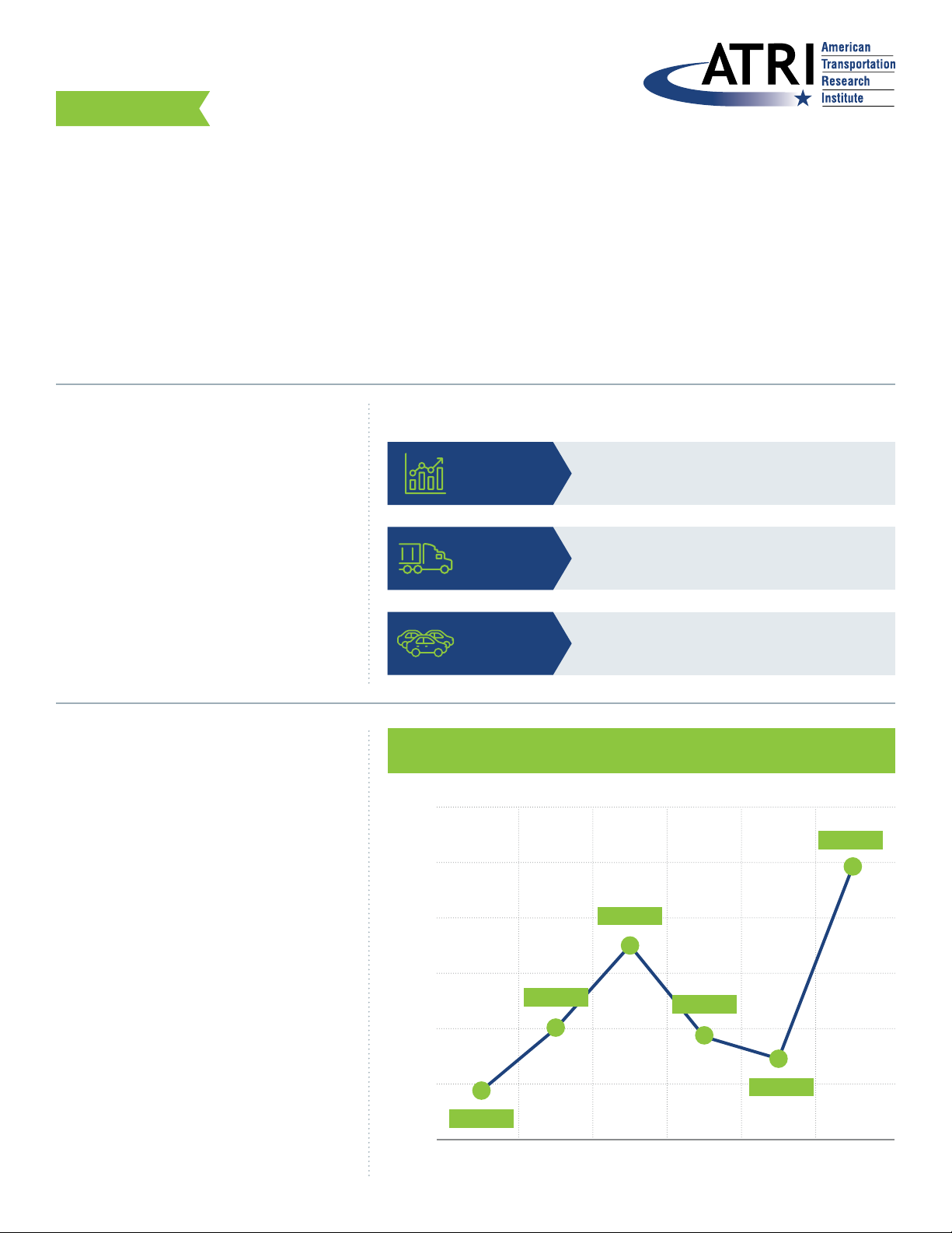


