Predicting Cryptocurrency Price Movements Using Machine Learning And Technical Indicators PDF Free Download
1 / 104/104
100%

Predicting Cryptocurrency Price Move-
ments Using Machine Learning And
Technical Indicators
Mike Miettinen
Master’s thesis
October 2025
Master’s Degree Programme in Artificial Intelligence and Data Analytics

Description
Miettinen, Mike
Predicting Cryptocurrency Price Movements Using Machine Learning And Technical Indicators
Jyväskylä: Jamk University of Applied Sciences, October 2025, 79 pages.
Degree Programme in Artificial Intelligence and Data Analytics. Master’s thesis.
Permission for open access publication: Yes
Language of publication: English
Abstract
Cryptocurrency markets are highly volatile and difficult to forecast, posing challenges for both investors and
researchers. This study investigated the use of machine learning models to predict short-term cryptocur-
rency price movements, using hourly data from Binance for five cryptocurrencies. A wide range of technical
indicators and candlestick features were employed as inputs, and both classification tasks (price direction)
and regression tasks (future high and low prices) were performed. Automated machine learning (AutoML)
with PyCaret was used to systematically evaluate a broad set of algorithms across different input window
sizes and prediction horizons.
The results showed that the Ridge Classifier generally outperformed other models in predicting price direc-
tion. For regression tasks at the one-hour horizon, Huber, Orthogonal Matching Pursuit, and Ridge regres-
sion achieved the lowest error rates, while Extra Trees gave better results for longer horizons. Incorporating
multiple previous hours of data improved model accuracy up to a threshold, after which additional lagged
features yielded little benefit. Prediction accuracy decreased substantially when extending the forecasting
horizon beyond one hour.
A key finding was that low error metrics, particularly mean absolute percentage error (MAPE), did not cor-
respond to genuine predictive power. Instead, the models often exhibited reactive behavior, replicating the
most recent price movement and effectively lagging behind by one time step. This limitation highlights the
difficulty of achieving forward-looking prediction in cryptocurrency markets.
The study concludes that while machine learning can provide systematic benchmarks and descriptive in-
sights into short-term price dynamics, its practical utility for live trading remains limited without additional
predictive signals. Future work should expand datasets, incorporate alternative data sources such as senti-
ment or blockchain network activity, explore deep learning architectures designed for sequential data, and
evaluate models in simulated environments to better assess their real-world applicability.
Keywords/tags (subjects)
Cryptocurrencies, technical analysis, trading, machine learning, supervised learning, classification, regres-
sion
Miscellaneous (Confidential information)
-

1
Contents
Terms.................................................................................................................................. 3
1 Introduction ................................................................................................................ 5
2 Ethical Considerations .................................................................................................. 6
3 Research Method (CRISP-DM) ...................................................................................... 7
4 Technical Analysis ........................................................................................................ 9
4.1 Moving Averages ............................................................................................................. 10
4.2 Trend Indicators .............................................................................................................. 13
4.3 Momentum Indicators .................................................................................................... 18
4.4 Volatility Indicators ......................................................................................................... 27
4.5 Volume Indicators ........................................................................................................... 29
5 Candlestick Patterns .................................................................................................. 32
6 Machine Learning ...................................................................................................... 33
6.1 Classification .................................................................................................................... 34
6.2 Regression ....................................................................................................................... 37
6.3 PyCaret ............................................................................................................................ 38
7 Prior Studies .............................................................................................................. 39
7.1 Technical Indicator Comparisons .................................................................................... 40
7.2 Machine Learning Model Comparisons .......................................................................... 42
8 Research Implementation .......................................................................................... 43
8.1 Business Understanding .................................................................................................. 44
8.2 Data Understanding & Preparation ................................................................................ 45
8.2.1 Feature Calculation ................................................................................................ 46
8.2.2 Candlestick Patterns .............................................................................................. 48
8.3 Modeling ......................................................................................................................... 50
8.3.1 Classification .......................................................................................................... 51
8.3.2 Regression .............................................................................................................. 61
9 Results ....................................................................................................................... 68
9.1 Classification .................................................................................................................... 68
9.2 Regression ....................................................................................................................... 73
9.3 Summary ......................................................................................................................... 77
2
10 Conclusion ................................................................................................................. 78
References ........................................................................................................................ 80
Appendices ....................................................................................................................... 88
Appendix 1. Technical indicators and corresponding parameters .......................................... 88
Appendix 2. Compared classification models in PyCaret ......................................................... 99
Appendix 3. Compared regression models in PyCaret ........................................................... 100
Appendix 4. Best performing classification models ............................................................... 101
Appendix 5. Best performing regression models ................................................................... 102
Figures
Figure 1. Diagram of CRISP-DM process ....................................................................................... 8
Figure 2. Example of Ichimoku Cloud graph ............................................................................... 15
Figure 3. Example of bullish and bearish candlesticks ................................................................ 32
Figure 4. Examples of candlestick patterns ................................................................................ 33
Figure 5. Code sample of PyCaret basic usage. .......................................................................... 39
Figure 6. Example of calculating features using Skender.Stock.Indicators library. .................... 46
Figure 7. C# implementation of the “Identical Three Crows” candlestick pattern. ................... 50
Figure 8. Profit rank distribution. ................................................................................................ 53
Figure 9. Confusion matrix of the best performing profit rank model. ...................................... 56
Figure 10. Classification accuracy by prediction horizon and lookback period. ......................... 58
Figure 11. Classification accuracy by prediction horizon and number of features. ................... 59
Figure 12. Error by prediction horizon and lookback period. ..................................................... 64
Figure 13. Error by prediction horizon and number of features. ............................................... 65
Figure 14. Confusion matrix of the best-performing tuned profit rank model on unseen data.70
Figure 15. Dogecoin candlestick chart with predicted profit ranks: green lines indicate high
predicted profitability, red lines indicate low predicted profitability. ....................................... 71
Figure 16. Confusion matrices of the high/low direction classification models with highest
accuracies. ................................................................................................................................... 72
Figure 17. Solana 12-hour high direction predictions: green lines indicate upward price movement
after 12 hours, red lines indicate downward movement. .......................................................... 73
Figure 18. Actual and predicted price of BTC from Aug 10th to Aug 16th in 2025. ..................... 75
Figure 19. Actual and predicted price of BTC on Aug 11th 2025. ............................................... 75
Figure 20. Actual and predicted price of DOGE on August 2025. ............................................... 76
Figure 21. Predicted profit rank distributions across cryptocurrencies and prediction horizons.77

3
Tables
Table 1. Confusion matrix in binary classification. ..................................................................... 35
Table 2. Studies comparing technical indicators. ....................................................................... 40
Table 3. Studies comparing machine learning models. .............................................................. 42
Table 4. Trading goals and means to achieve them. .................................................................. 44
Table 5. Five major cryptocurrencies selected to represent diverse market segments and use cases.
..................................................................................................................................................... 45
Table 6. Engineered features capturing profit potential and crossover trends. ........................ 47
Table 7. Candlestick characteristics translated into numerical measures and formulas. .......... 48
Table 8. Translation of Bulkowski’s qualitative terms into percentile-based comparisons. ...... 49
Table 9. Lookback windows, prediction horizons, and feature counts used in experiments. ... 50
Table 10. Definition of classification and regression target variables and their value ranges. .. 51
Table 11. Most frequent classification target values and their relative shares for each
cryptocurrency. ........................................................................................................................... 52
Table 12. Top-performing classification models and parameter settings identified during
preliminary evaluation. ............................................................................................................... 53
Table 13. Best classification scores using a zero-hour lookback period and all features. .......... 60
Table 14. Baseline regression model performance (MAPE) for High and Low price predictions.61
Table 15. Top-performing regression models and parameter settings identified during preliminary
evaluation.................................................................................................................................... 62
Table 16. Best regression model scores for each cryptocurrency using all features and any lookback
period. ......................................................................................................................................... 66
Table 17. Classification accuracies of tuned models across cryptocurrencies and prediction
horizons. ...................................................................................................................................... 68
Table 18. Regression error rates of tuned models across cryptocurrencies and prediction horizons.
..................................................................................................................................................... 74
Terms
BR Bayesian Ridge
DNN Deep Neural Network
DT Decision Tree
EN Elastic Net
ET Extra Tree
GB Gradient Boosting
4
GBM Gradient Boosting Machine
KNN K-Nearest Neighbors
KR Kernel Ridge
LR Linear Regression
LSTM Long Short Term Memory
MAPE Mean average percentage error
ML Machine learning
MLP Multi-Layer Perceptron Neural Network
NN Neural Network
OHLC Open, high, low and close prices of financial instruments
OLS Ordinary Least Squares
RF Random Forest
RNN Recurrent Neural Network
RR Ridge Regression
SMA Simple moving average
SGD Stochastic Gradient Descent
SVM Support Vector Machine
SVR Support Vector Regression

5
1 Introduction
Cryptocurrency markets are characterized by extreme volatility, rapid fluctuations, and sensitivity
to both internal and external factors. These dynamics create substantial risks for investors, but
also opportunities for profit if price movements can be anticipated with sufficient accuracy. Tradi-
tional forecasting methods, often designed for more stable financial markets, struggle to capture
the nonlinear and fast-changing behaviour of cryptocurrencies.
Machine learning (ML) has emerged as a promising alternative, offering the ability to process large
volumes of market data, identify hidden patterns, and adapt to complex temporal structures. In
financial research, ML methods have been applied to tasks ranging from trend classification to
price level prediction, with varying degrees of success. Within the cryptocurrency domain, their
appeal lies in the potential to transform raw technical indicators into actionable trading signals.
This thesis investigates the use of ML models for short-term cryptocurrency forecasting. A wide
range of technical indicators and candlestick patterns are employed as inputs, and both classifica-
tion (directional movement) and regression (price level prediction) tasks are explored. Automated
machine learning (AutoML) is applied to systematically evaluate multiple models across several
cryptocurrencies, lookback window sizes, and prediction horizons.
The study is guided by the following research questions:
• Is it possible to identify favorable times to enter or exit the market using ML models based
on technical indicators?
• Can ML models estimate reasonable buy and sell price levels based on historical price pat-
terns?
• Which ML models perform best in classification and regression tasks for cryptocurrency
price prediction?
• Does including additional lagged data improve predictive performance?
• How does prediction horizon length affect model performance and predictive reliability?
• Do predictive patterns or model performances differ systematically across cryptocurren-
cies?
6
In addition to benchmarking model performance, the study also critically examines whether the
models demonstrate genuine predictive ability or merely reactive behaviour. While low error rates
can suggest high accuracy, they may also reflect a tendency to replicate recent price movements
rather than anticipate future changes. Recognizing and articulating this distinction is central to
evaluating the true utility of ML for cryptocurrency forecasting.
By addressing these questions, the thesis aims to contribute both methodologically and practi-
cally: providing systematic benchmarks of ML model performance in cryptocurrency markets and
clarifying the extent to which such models can support forward-looking decision-making in one of
the most dynamic domains of modern finance.
2 Ethical Considerations
Ethical considerations in this research focused on the responsible use of data, the transparency of
methods, and the interpretation of results. All used data was obtained from public sources and
was available without a charge. Ethical questions related to data were addressed by ensuring the
sources were referenced appropriately and that the research is reproducible. Research transpar-
ency and integrity were ensured by describing data preprocessing, technical indicator calculation
and ML model selection in sufficient detail so the reader could evaluate research reliability and
suitability of the methods.
Using ML for financial predictions involves its own specific ethical risks. Predictive models may
lead to incorrect assumptions or unrealistic expectations if their limitations aren’t understood.
These limitations were critically considered, and results were presented in a manner that cannot
be interpreted as trading advice or guiding decision making. This approach aimed to prevent mis-
leading conclusions and ensure the research objectives stay within scientific and analytical con-
text.
Ethical responsibility was also present in critical reflection and openness. Potential error sources
were identified, and model limitations were evaluated. Work was conducted honestly, transpar-
ently, and responsibly, ensuring all stages of research are assessable and reproducible.
7
3 Research Method (CRISP-DM)
The Cross-Industry Standard Process for Data Mining (CRISP-DM) is a widely used methodological
framework developed in the late 1990s to provide a structured and repeatable approach for data
mining and ML projects. It is designed to guide a project from the initial definition of the problem
through to the delivery of results, ensuring that all relevant aspects are systematically addressed.
The framework is cyclical and iterative, allowing researchers to move back and forth between
phases as needed, which makes it especially suitable for exploratory and experimental research.
(Wirth & Hipp, 2000)
CRISP-DM consists of six phases, each serving a distinct role in the data mining and ML workflow
as shown in Figure 1.

8
Figure 1. Diagram of CRISP-DM process (Jensen, 2012).
Business Understanding
This phase focuses on clarifying the objectives and requirements of the project from a business or
research perspective. The key task is to define the problem, establish success criteria, and trans-
late these into a data mining or ML problem. (Wirth & Hipp, 2000)
Data Understanding
The second phase involves collecting, exploring, and describing the data. It includes assessing data
quality, identifying potential issues, and forming initial hypotheses. (Wirth & Hipp, 2000)
9
Data Preparation
Often the most time-consuming phase, data preparation involves cleaning and transforming the
raw data into a form suitable for modeling. Typical activities include handling missing values, cre-
ating new features, and selecting relevant subsets of data. (Wirth & Hipp, 2000)
Modeling
In this phase, suitable modeling techniques are chosen and applied to the prepared dataset. It in-
volves building, calibrating, and experimenting with different algorithms, as well as adjusting pa-
rameters to find the best-performing models. (Wirth & Hipp, 2000)
Evaluation
The fifth phase assesses whether the developed models meet the defined objectives. This involves
both technical validation (e.g., prediction accuracy, precision, recall) and alignment with the initial
problem statement. (Wirth & Hipp, 2000)
Deployment
The final phase is about putting the results into use and communicating findings. In business set-
tings this may involve implementing a live system, while in academic contexts it typically means
reporting results, interpreting outcomes, and discussing implications. (Wirth & Hipp, 2000)
4 Technical Analysis
Technical analysis in trading aims to forecast future price movements by analyzing historical mar-
ket data. It utilizes past prices to project future movements, assuming that prices integrate all
known market factors and follow identifiable patterns (Brown & Jennings, 1989). This method,
widely used across financial markets such as foreign exchange, becomes particularly useful for
short-term predictions. Many see technical analysis as self-reinforcing due to its common use (Tay-
lor & Allen, 1992).

10
Within the field, countless patterns and signals have been crafted to support technical analysis in
trading. Indicators may focus on identifying current market trends, including critical points like
support and resistance, or assessing the momentum and durability of a trend. Key technical indica-
tors and patterns often utilize trendlines, channels, moving averages, and momentum measures.
Broadly, technical analysts evaluate indicators related to price movements, chart formations, vol-
ume and momentum metrics, oscillators, and levels of support and resistance. (Hayes, 2024).
4.1 Moving Averages
Simple Moving Average
Simple Moving Average (SMA) is one of the most fundamental and widely used technical indica-
tors. SMA calculates the average price during a specific time period. It’s delayed and trend follow-
ing indicator which smoothens the price data and helps to identify the direction of current trend
and possible support and resistance levels. (Colby, 2003). SMA is calculated using formula 1
(1)
where n is the number of values in the selected time period (Banton, 2024).
Weighted Moving Average
Weighted Moving Average (WMA) adds weight to moving average. WMA treats the latest values
as more significant than older values. This makes WMA more sensitive and faster in reacting to
price changes. WMA is delayed and trend following like SMA. (Colby, 2003). WMA is calculated by
adding linearly increasing weight to all data points
(2)
where n is the number of values in the selected time period and w linearly increasing weight (Ban-
ton, 2024).

11
Exponential Moving Average
Exponential Moving Average (EMA) is similar to WMA, but the weights diminish exponentially the
older the values are (Colby, 2003). The value is calculated iteratively using a smoothing factor (α)
(3)
where n is the number of values in the selected time period (Banton, 2024).
Double Exponential Moving Average
Double Exponential Moving Average (DEMA) is a modified version of the EMA, and its primary goal
is to reduce lag compared to traditional moving averages. DEMA aims to react faster to price
changes and give earlier signals of trend changes. (Colby, 2003). EMA is calculated using formula 4
(4)
where n is the selected time period (TrendSpider, n.d. -a).
Hull Moving Average
Hull Moving Average (HMA), developed by Alan Hull, is designed to significantly reduce lag and en-
hance sensitivity compared to traditional moving averages. HMA aims to provide a smoother and
faster moving average, which reacts fast to price changes while reducing signal noise. HMA is cal-
culated using formula 5
(5)

12
where n is the selected time period (Fidelity, n.d. -a).
Kaufman's Adaptive Moving Average
Kaufman's Adaptive Moving Average (KAMA), developed by Perry Kaufman, is a dynamic and
adaptive moving average. KAMA’s essential feature is its ability to adjust sensitivity based on mar-
ket volatility. On vertical market KAMA slows down its reactivity whereas on trending market it
speeds up reactivity to follow price more closely. This adaptive nature allows KAMA to reduce lag
on strong trends and filter noise on vertical markets. KAMA is calculated using formula 6
(6)
where SCfast and SCslow are constants which control the smoothing level and n is the selected time
period. (StockCharts, n.d. -a)
Smoothed Moving Average
Smoothed Moving Average (SMMA) is a hybrid between SMA and EMA. SMMA aims to provide an
extremely smooth line of the price data, and it reacts slower to price changes than most other
moving averages. SMMA is especially useful in identifying long term trends and filtering market
noise. (De Turck, 2024). SMMA is calculated using formula 7
(7)
where n is the number of periods (Sourcetable, n.d.)

13
4.2 Trend Indicators
Aroon Oscillator
Aroon Oscillator is a trend following oscillator which is used to identifying trend direction and
strength. Aroon Oscillator measures time passed since previous highest high and lowest low.
Aroon oscillator is calculated using formula 8
(8)
where n is the number of values in the selected time period, periodshigh is the number of periods
since last highest high and periodslow the number of periods since last lowest low. (Colby, 2003)
Average Directional Index
Average Directional Index (ADX) is a technical indicator developed by J. Welles Wilder Jr. to evalu-
ate trend strength regardless of its direction. It helps to specify whether there’s a dominant trend
in the market. ADX is delayed and trend following indicator, and it oscillates between 0 and 100.
ADX calculation is based on True Range (TR) and Directional Movement (DM). (Pring, 2014). ADX is
calculated using formula 9
(9)

14
where n is the number of values in the selected time period (MotiveWave, n.d. -a).
ATR Trailing Stop
ATR Trailing Stop is used to set dynamic stop-loss levels which adjust to market volatility. It’s
based on Average True Range (ATR) which measures volatility. ATR Trailing Stop is a trend follow-
ing stop-loss method which follows price to the direction of trend and secures profits while also
protecting from losses. ATR Trailing Stop is calculated using formula 10
(10)
where n is the selected time period and Factor (usually 2 or 3) is a multiplier which is set according
to strategy and risk tolerance. (StockCharts, n.d. -b) ATR formula is shown in Equation (38.
Chandelier Exit
Chandelier Exit is a volatility based stop-loss which is designed specifically for trend following trad-
ing strategies. Chandelier Exit aims to set a dynamic trailing stop-loss level which adjusts to market
volatility and follow price to trend direction. Chandelier Exit strives to secure profits during rising
trend and limit losses on falling trend. Chandelier Exit is calculated using formula 11
(11)
where n is selected time period and Multiplier (typically 3) is selected based on strategy and risk
tolerance. (Groette, 2024).
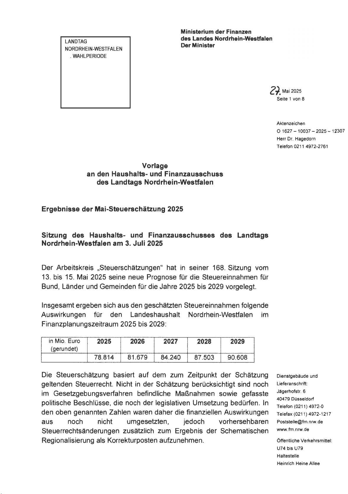
Ichimoku Cloud
Ichimoku Kumo Hyo also known as Ichimoku Cloud (IC), is developed by Goichi Hosoda. It’s de-
signed to provide a comprehensive view on market dynamics at a glance. IC is a trend following

15
indicator which visualizes support and resistance levels, momentum and trend direction and pro-
vides trading signals. IC is formed of five main components which together form a cloud on top of
the price chart.
- Base line (Kijun-sen) is the average of highest and lowest price within a long time period
- Conversion line (Tenkan-sen) is the average of highest and lowest price within a short time period
- Leading span A (Senkou span A) is the average of base line and conversion line moved forward by
26 periods
- Leading Span B (Senkou span B) is the average of highest and lowest price within even longer time
period moved forward by 26 periods
- Lagging span line (Chikou span) is current close price moved backward 26 periods. (Thompson,
2025).
Figure 2 demonstrates how IC lines form clouds above candlestick graph.
Figure 2. Example of Ichimoku Cloud graph (Bybit Learn, 2021).
McGinley Dynamic
McGinley Dynamic, developed by John R. McGinley, is a dynamic moving average which is de-
signed to overcome the limitations of SMA and EMA. McGinley Dynamic’s primary goals are to re-
duce lag and enhance responsiveness to price changes compared to traditional moving averages.
Indicator adjusts its smoothing factor automatically making it move faster on trending market on
slower on vertical market. McGinley Dynamic is calculated using formula 12

16
(12)
where n is selected time period and k is a factor which is usually constant 0.6. (Twomey, 2022).
Moving Average Envelopes
Moving Average Envelopes (MAE) is formed of two bands which are drawn percentual offset
above and below moving average. Moving Average Envelopes is designed to visualize normal
movement of the price and identify overtrading and overselling states. It is assumed the price will
typically stay between the bands and movement outside could indicate exceptional conditions or
starting trends. MAE is calculated using formula 13
(13)
where n is selected time period and Offset percentual offset. (Fidelity, n.d. -b)
Parabolic Stop and Reverse
Parabolic Stop and Reverse (Parabolic SAR), developed by J. Welles Wilder Jr., is used to identify
trend direction and produce trading signals. Parabolic SAR is represented with dots above and be-
low the price candlesticks. When dots are below the prices, the trend is rising. When the dots are
above the prices, the trend is falling. Parabolic SAR is calculated using formula 14
(14)
where EP is an extreme point, which is the highest price on rising trend and the lowest price on
falling trend. The AF is an acceleration factor which starts usually from 0,02 and increases by 0,02
every time a new EP is reached until a maximum value (usually 0,2) is reached. (Wilder, 1978)

17
Vortex Indicator
Vortex Indicator (VI), developed by Etienne Botes and Douglas Siepman, is used to identify trend
direction and strength. VI is formed of two lines, VI+ and VI-, which measure positive and negative
trend movements respectively. VI is calculated using formula 15
(15)
where n is the selected time period and TR True Range (formula 39). (Chen, 2022 -a)
Williams Alligator
Williams Alligator, developed by Bill Williams, is a trend following indicator aimed to identify mar-
ket trends. The indicator is formed of three moving averages called Jaw, Teeth and Lips. These
lines form the following patterns
• Sleeping alligator is formed when all three lines are close to each other. It indicates market being in
vertical movement. I.e. markets don’t have a clear trend.
• Waking alligator is formed when lines are starting to spread. It indicates the start of a new trend.
• Eating alligator is formed when lines are widely spread and in order. It indicates strong and lasting
trend.
All lines use the same formula 16
(16)
where n and offset are different for each line usually 13, 8, and 5 for n and 8, 5, and 3 for offset in
order jaw, teeth, lips. (FBS, n.d.)
18
4.3 Momentum Indicators
Absolute Price Oscillator
Absolute Price Oscillator (APO) is a momentum oscillator which helps identify trend direction,
strength and possible turning points. APO is calculated by subtracting long period moving average
from short period moving average.
(17)
APO interpretation is based on the value itself, crossing the zero line and divergence. Positive val-
ues indicate rising momentum and negative values falling momentum. Crossing the zero line indi-
cates momentum gaining strength in similar direction. When the price reaches new low, but simi-
lar change isn’t seen in APO it indicates a falling trend getting weaker and potentially trend turning
upwards. Similarly, when price reaches a new high, but same cannot be seen in APO, it indicates
the opposite. (TrendSpider, n.d. -b)
Awesome Oscillator
Awesome oscillator (AO) is a momentum oscillator primarily aimed to measure momentum by
comparing short term momentum to long term momentum. It aims to identify whether the mo-
mentum is rising or falling and giving signals of possible trend changes. AO is a popular indicator in
identifying trend strength and possible trend reversals. AO is calculated using formula 18
(18)
AO crossing above zero indicates starting of an upward trend or it is getting stronger. The opposite
is true for AO crossing below zero. (AvaTrade, n.d. -a)
Balance of Power
Balance of Power (BOP) is used to measure the power ratio between buyers and sellers during
specific time period. Indicator strives to quantify which party is controlling the market. BOP is not
trend following or momentum indicator in a traditional sense, but it’s more like an oscillator which

19
depicts price movement dynamics within a time period. It’s useful in identifying possible changes
in trends and verifying the direction of the price movement. BOP is calculated using formula 19
(19)
BOP usually oscillates between -1 and +1. Interpretation is based not only on the value, but also on
the movement around zero. Positive BOP implies buyers have more control. The closer the value is
to +1 the stronger the buyers have controlled the market. Negative BOP indicates sellers control-
ling the market. Similarly, the closer the values are to -1 the stronger the sellers have been con-
trolling the market. When BOP crosses above the zero line, it indicates buyers are getting stronger
and there is the possibility for a rising trend. Similarly crossing below the zero line indicates sellers
gaining strength and possibility of a down trend. (TradingView, n.d. -a)
Chande Momentum Oscillator
Chande Momentum Oscillator (CMO) is used to measure the strength of the momentum and iden-
tify overbuying and overselling scenarios. CMO differs from Relative Strength Index in considering
also rising and falling periods in momentum calculation where RSI focuses primarily on closing
price in relation to fall. CMO oscillates between -100 and +100. CMO is calculated using formula 20
(20)
where Su is the sum of positive price changes and Sd the sum of negative price changes during the
time period. Positive CMO indicates rising periods having stronger momentum than falling periods
implying rising momentum in the market. The closer the value is to +100 the stronger the rising
momentum is. When CMO crosses above the zero line, it could indicate rising momentum gaining
strength and possibly a good time to enter the market. Negative CMO values and crossing below
the zero line indicate the opposite i.e. falling momentum being stronger and possibly a good time
to exit the market. (Hayes, 2022)

20
Commodity Channel Index
Commodity Channel Index (CCI) is a technical analysis indicator that measures the current price of
a security relative to its average price over a given period. Developed by Donald Lambert in 1980,
it was originally created to identify cyclical turns in commodity markets, but is now widely used for
stocks, currencies, and other securities. CCI is calculated using formula 21
(21)
where n is the selected time period. (TradingView, n.d. -b)
Commodity Selection Index
Commodity Selection Index (CSI) is a technical momentum indicator used to help traders identify
which commodities are most suitable for short-term trading. CSI measures a commodity's trending
strength and volatility in relation to the costs of trading it, such as margin requirements and com-
missions. A higher CSI value indicates that a commodity has strong trending and volatility charac-
teristics, making it potentially more profitable for short-term trading. CSI is calculated using for-
mula 22
(22)
where ADX is Average Directional Index (formula 9) and ATR Average True Range (formula 38).
(Banton, 2022)

21
Detrended Price Oscillator
Detrended Price Oscillator (DPO) is a technical indicator used to eliminate the long-term trend
from a security's price data. By doing so, it helps traders to more clearly identify and analyze un-
derlying short-term price cycles and overbought/oversold conditions. DPO is calculated using for-
mula 23
(23)
where n is the selected time period. (TradingView, n.d. -c)
Elder Ray Index
Elder Ray Index is a technical analysis indicator developed by Alexander Elder that measures the
amount of buying and selling pressure in the market. It's designed to see through price move-
ments to determine the strength of the competing groups of bulls (buyers) and bears (sellers). The
indicator consists of two separate histograms, Bull Power and Bear Power, which are plotted be-
low the price chart. Elder Ray Index is calculated using formula 24
(24)
where n is the selected time period. (Colby, 2003)
Gator Oscillator
Gator Oscillator (GO) is a technical analysis tool created by Bill Williams. Gator Oscillator is used to
complement the Alligator Indicator by providing a clearer, histogram-based visual representation
of the trend's strength and direction. GO is displayed as a dual histogram, with bars plotted both
22
above and below a zero line. It measures the convergence and divergence of the three moving av-
erages that make up the Alligator Indicator, metaphorically described as the Alligator's Jaw, Teeth,
and Lips. GO is calculated using formula 25
(25)
where Lips, Teeth and Jaw are values from Williams Alligator (formula 16). (MotiveWave, n.d. -b)
Moving Average Convergence / Divergence
Moving Average Convergence / Divergence (MACD) is one of the most popular and versatile tech-
nical indicators. The primary goals of MACD are to identify trend direction, measure strength of
the momentum and detect possible trend reversals. MACD forms of two lines, MACD line and sig-
nal line, and a histogram which together provide a comprehensive view on market dynamics.
MACD is calculated using formula 26
(26)
where short, long, and signal_periods are selected period lengths, usually 12, 26, and 9 respec-
tively. (Interactive Brokers, n.d.)
On Balance Volume
On Balance Volume (OBV) is used to measure buying and selling pressure on financial markets. The
main idea of OBV is that volume should precede price. OBV aims to detect whether the volume
accumulates during rising or falling periods and gives cues of potential price movements. OBV is
calculated by adding volume on rising periods and subtracting on falling periods. OBV is calculated
using formula 27

23
(27)
(Fidelity, n.d. -c)
Percentage Price Oscillator
Percentage Price Oscillator (PPO) is used to measure momentum changes and identify overtrading
and overselling states. PPO represents the percentual difference between two moving averages.
PPO is calculated using formula 28
(28)
where long and short are selected time periods. (StockCharts, n.d. -c)
Rate of Change
Rate of Change (ROC) is used to measure price change speed during a time period. ROC is a mo-
mentum oscillator which indicates how much price has changed from previous point in time. ROC
aims to identify momentum changes, overtrading and overselling states and potential trend rever-
sals. ROC is calculated using formula 29
(29)
where n is the selected time period. (Kirkpatrick & Dahlquist, 2010)
Relative Strength Index
Relative Strength Index (RSI), developed by J. Welles Wilder Jr., is a widely used momentum oscil-
lator. RSI’s primary goal is to measure the speed and size of the price change so that overtrading
and overselling states could be evaluated. RSI aims to identify whether momentum is increasing or

24
decreasing and give clues about possible trend changes. RSI oscillates between 0 and 100. RSI is
calculated using formula 30
(30)
where n is the selected time period. (Colby, 2003)
Schaff Trend Cycle
Schaff Trend Cycle (STC) is designed to combine the best parts of cycle analysis and measuring mo-
mentum. It was developed by Doug Schaff. STC is an oscillator which aims to identify both trend
direction and it’s cyclic nature by giving signals of potential trend changes, overtrading and over-
selling states. STC oscillates between 0 and 100. STC is calculated using formula 31
(31)
where %DMACD and %KMACD are stochastic (formula 32) values of MACD (formula 26). (HowToTrade,
2023)
Stochastic Oscillator
Stochastic Oscillator is a momentum oscillator which is widely used to identify overtrading and
overselling states and predict potential trend reversals. Stochastic Oscillator is based on the obser-
vation that during a rising trend, prices tend to close near high and during a falling trend near low.
Stochastic Oscillator measures the position of current close in relation to price range within a spe-
cific time period. Stochastic Oscillator forms of two lines, %K and %D, which oscillate between 0
and 100. Stochastic Oscillator is calculated using formula 32

25
(32)
where n is the selected time period. (Kirkpatrick & Dahlquist, 2010)
Stochastic RSI
Stochastic RSI (StochRSI) is a technical indicator created by applying the Stochastic Oscillator for-
mula to the Relative Strength Index (RSI) values instead of a security's price data. It’s designed to
be more sensitive and generate more trading signals than the traditional RSI. StochRSI is calculated
using formula 33
(33)
where n is the selected time period. (Corporate Finance Institute, n.d.)
Triple Exponential Moving Average
Triple Exponential Moving Average (TRIX) is a momentum indicator which measures percentual
change speed from thrice smoothened EMA. TRIX aims to filter out short term noise and focus on
long term, more significant trend changes. TRIX is calculated using formula 34
(34)
where n is the selected time period. (Chen, 2022 -b)

26
True Strength Index
True Strength Index (TSI) is a momentum oscillator which aims to measure trend direction and
strength by filtering price noise. TSI is designed to be smoother and less prone to false signals than
traditional oscillators, such as RSI. TSI is especially useful in identifying trend direction, overtrading
and overselling states, and identifying divergences between price and momentum. TSI oscillates
around zero line. TSI is calculated using formula 35
(35)
(TradingView, n.d. -e)
Ultimate Oscillator
Ultimate Oscillator (UO) is a momentum oscillator which aims to enhance signal reliability by re-
ducing divergence traps. UO calculates the weighted average of the momentum using three differ-
ent time periods. UO aims to provide more thorough view on market buying and selling pressure
and identify potential overtrading and overselling states. (Colby, 2003). UO is calculated using for-
mula 36
(36)
Where short, middle and long are selected time periods (commonly 7, 14 and 28) shortest to long-
est. (TradingView, n.d. -d)

27
Williams’ Percent Range
Williams Percent Range (%R) is a momentum oscillator developed by Larry Williams. %R measures
current closing price in relation to the range between highest and lowest price within a specific
time period. %R is designed to identify overtrading and overselling states in the market and it aims
to provide cues of potential price reversals and corrections. %R oscillates between -100 and 0. %R
is calculated using formula 37
(37)
where n is the selected time period. (Kirkpatrick & Dahlquist, 2010)
4.4 Volatility Indicators
Average True Range
Average True Range (ATR) is a volatility indicator used to measure price change range within a
given time period. ATR doesn’t measure trend direction like many other indicators, but only the
degree of volatility. ATR is useful in risk management, setting stop-loss levels and identifying vola-
tility changes in the market. ATR is calculated using formula 38
(38)
where n is the selected time period. (Colby, 2003)
Bollinger Bands
Bollinger Bands (BB), developed by John Bollinger, is widely used to measure volatility and identity
possible overtrading and overselling states. Bollinger Bands are made of three lines which are
drawn on top of a price chart.
28
• Middle line is simple moving average (SMA) over selected periods
• Upper line is two standard deviations above middle line
• Lower line is two standard deviations below the middle line
The area between upper and lower lines represents the price range which is expected to contain
most of the price movements. Line distance from the middle line adjusts to volatility change.
When volatility increases the lines move further from the middle line and when volatility de-
creases, they move closer. (Colby, 2003)
Donchian Channels
Donchian Channels, developed by Richard Donchian, is an indicator based on volatility which
draws three lines on top of price graph.
• Upper Channel is the highest price during selected time period
• Lower Channel is the lowest price during selected time period
• Middle Line is the average of upper and lower channels
Price crossing above upper channel indicates potential rising trend and crossing below lower chan-
nel falling trend. Upper channel rising while lower channel stays steady could also indicate rising
trend. Similarly lower channel falling while upper channel stays steady could indicate a falling
trend. (AvaTrade, n.d. -b)
Keltner Channels
The Keltner Channel is a technical analysis indicator that measures a security's volatility and helps
to identify trends and potential reversal points. It is a type of envelope or channel indicator that
uses volatility to define its boundaries. The channel is plotted above and below a central moving
average, creating a visual representation of price action relative to its typical range. Keltner Chan-
nel consists of three lines, which are calculated using the Exponential Moving Average (EMA) and
the Average True Range (ATR). The ATR is used to measure volatility and determine the width of
the channel.
• Middle Line: A standard EMA of the closing price, typically over 20 periods.
• Upper Band: The middle line plus a multiple of the ATR.
• Lower Band: The middle line minus a multiple of the ATR.

29
The multiple is a user-defined factor. (Colby, 2003)
STARC Bands
STARC Bands, short for Stoller Average Range Channels, are a volatility-based technical analysis
indicator used to determine price channel boundaries. Developed by Manning Stoller, the indica-
tor plots a channel around a Simple Moving Average (SMA), with the width of the channel deter-
mined by the Average True Range (ATR). STARC Bands are calculated using formula 39
(39)
where n is the selected time period, TR is true range (formula 38) and k the factor (typically 2).
(Quantified Strategies, 2024)
4.5 Volume Indicators
Accumulation Distribution Line
Accumulation Distribution Line (ADL) is a volume-based indicator which combines price and vol-
ume data to evaluate the pressure between buyers and sellers. ADL aims to identify whether the
volume is accumulating or distributing in a specific time period. ADL strives to amplify trends and
detect divergences between price and volume which could give cues of potential trend changes.
ADL is calculated using formula 40
(40)

30
Rising ADL indicates accumulation i.e. pressure being greater on buyers’ side and typically indicat-
ing rising trends. Falling ADL indicates distribution, i.e. pressure being greater on sellers’ side and
indicating falling trends. (TradingView, n.d. -f)
Chaikin Money Flow
Chaikin Money Flow (CMF), developed by Marc Chaikin, is a volume-based indicator used to meas-
ure buying and selling pressure. CMF aims to identify which side, buyers or sellers, has more con-
trol on financial markets based on volume and price movement. CMF is represented as an oscilla-
tor which moves between -1 and +1. It’s developed to give signals of potential trend changes and
amplifying existing trends. CMF is calculated using formula 41
(41)
where n is the selected time period. (TradingView, n.d. -g)
Chaikin Oscillator
Chaikin Oscillator (CO) is a technical analysis indicator that measures the momentum behind a se-
curity's Accumulation/Distribution Line (ADL). It was developed by Marc Chaikin, the same creator
as the Chaikin Money Flow (CMF). The oscillator is a tool for identifying changes in momentum,
which can signal potential trend reversals in a security's price. CO is calculated using formula 42
EMA(ADL, short) – EMA(ADL, long)
(42)
where short and long are selected time periods (typically 3 and 10). (Investopedia, n.d.)
Force Index
Force Index is designed to measure the strength of price movement by combining price direction,
change and volume. Force Index aims to quantify buyers and sellers’ actual power on the market.
It’s useful in confirming trends, identifying possible trend reversals. Force Index is an oscillator
which swings around zero. Force Index is calculated using formula 43

31
(43)
where n is the selected time period. (StockCharts, n.d. -d)
Money Flow Index
Money Flow Index (MFI) is used to measure invested money’s flow to a security. MFI is a momen-
tum oscillator which factors in price and volume aiming to identify overselling and overbuying sce-
narios. MFI is based on Relative Strength Index, but it adds weighing by volume making it more
comprehensive measure on market dynamics. MFI oscillates between 0 and 100. MFI is calculated
using formula 44
(44)
where n is the selected time period. (TradingView, n.d. -h)
Percentage Volume Oscillator
Percentage Volume oscillator (PVO) is used to analyze volume momentum. PVO measures the per-
centual difference between short and long EMA. It’s similar to the Percentage Price Oscillator but
uses volume instead of price. The primary goal of PVO is to detect changes in the strength of vol-
ume momentum and provide clues of potential trend changes from the volume perspective. PVO
oscillates around zero. PVO is calculated using formula 45

32
(45)
where nshort and nlong are selected time periods. (StockCharts, 2024)
5 Candlestick Patterns
Financial instrument price movements are commonly visualized using candlestick graphs. A single
candlestick represents the open, high, low, and close (OHLC) prices of a certain time frame. Can-
dlesticks are formed of a box which shows the range between the open and close prices. Lines
above and below the box, known as wicks, show the high and low prices. The color of the candle-
stick indicates the direction of the price. Green is commonly used to indicate rising (bullish) prices
and red to indicate falling (bearish) prices. Examples of bullish and bearish candlesticks are shown
in Figure 3.
Figure 3. Example of bullish and bearish candlesticks (TradeBrigade, n.d.).
One or more candlesticks with certain characteristics and relations to others form commonly
recognizable patterns which are claimed to predict changes in the price movement. Various
sources list different patterns, and the total number of patterns is most likely unknown. E.g.
Bulkowski (2008) lists 103 patterns. Examples of candlestick patterns are shown in Figure 4.

33
Figure 4. Examples of candlestick patterns (TradeBrigate, n.d.).
6 Machine Learning
ML is an essential part of artificial intelligence and focuses on developing systems and algorithms
which can learn from data without being explicitly programmed for a specific task. Instead of pro-
grammers specifying strict rules to solve a problem, ML models learn these rules by themselves by
analyzing a great amount of data and identifying patterns from it. (Mitchell, 1997)
The core of ML is utilizing data. The models are trained using extensive sample data, which is
called training data. During the training process the model aims to find hidden connections and
structures within the data. The goal of the training is to get the model capable of generalizing
learned rules and applying them to new, unseen data and make precise predictions, classifications
and similar conclusions. (Mitchell, 1997) ML methods can be divided into three main categories:
supervised learning, unsupervised learning and reinforcement learning (Goodfellow et al., 2016).
In supervised learning model is given sample data which contains both the inputs and the corre-
sponding labels. Model aims to learn a function which maps the inputs to the labels. Typical super-
vised learning tasks include classification, where the model aims to predict a categorical variable
(e.g. whether an email is spam or not), and regression which aims to predict a continuous variable
(e.g. the price of an apartment). (Goodfellow et al., 2016)
34
In unsupervised learning the training data doesn’t contain predefined labels or “correct” answers.
The purpose of the model is to independently find hidden structures, groups or rules. Common ex-
ample of unsupervised learning is clustering, where the data is divided into groups, each contain-
ing observations with similar features. (Goodfellow et al., 2016)
In reinforcement learning the agent learns to function in its environment through interactions. The
agent makes decisions and gets positive or negative feedback from the environment. The agent
aims to learn a strategy which maximizes the long-term reward. Reinforcement learning is used
robotics, games, and autonomous systems. (Goodfellow et al., 2016)
6.1 Classification
Classification is one of the essential tasks in ML. Classification aims to predict categorical variables
(classes) from previously seen marked data. Typically, classification models are trained using data
where each observation consists of features and corresponding correct class, called label. The goal
is to get the model to generalize seen patterns to be able to do precise classifications also for new,
unseen data. (Bishop, 2006).
Classification tasks can be divided into two main groups: binary classification, where there are two
possible classes (e.g. true and false), and multinomial classification, where there are more possible
classes (e.g. identifying plant species). (Goodfellow et al., 2016). In the context of predicting cryp-
tocurrency price movements, a possible classification task could be predicting whether the price
goes up or down during the selected time period.
Multiple different algorithms are used in classification, and they differ in complexity and suitability
for different kinds of scenarios. Logistic regression is especially suitable for binary classification
and is based on logistic function, which models the probability of given class (Hastie et al., 2009).
Decision trees build hierarchical structures, where a decision is made in all nodes based on some
feature. Leaf nodes contain the final classes. Decision trees are easy to interpret and work well
with categorical data, but overfitting can happen if the model complexity isn’t limited. (Bishop,
2006). Random forests are ensemble methods, which form a great number of decision trees and
merge their decision by voting. This enhances accuracy and reduces the risk of overfitting com-
pared to a single decision tree. (Breiman, 2001). K-Nearest neighbors (KNN) is a non-parametric

35
method, where the class of a datapoint is determined by plurality vote of its neighbors. The goal is
to assign a class which is the most common within its k neighbors. (Hastie et al., 2009). Support
vector machines (SVM) aim to find hyperplanes which separate the classes by maximal margin.
SVMs works especially well on high-dimensional data and can be extended to nonlinear problems
by using kernel functions. (Cortes & Vapnik, 1995). Naïve Bayes classifier is based on Bayes’ theo-
rem and assumes features’ conditional independence. Although the assumption is unrealistic, the
method works well with text classification and email spam detection. (Mitchell, 1997). Neural net-
works are formed of multiple layers of artificial neurons, which can learn complex non-linear func-
tions. They are especially suitable for large and high-dimensional data, such as images or natural
language. The downside is greater processing power needs and harder interpretation. (Goodfellow
et al., 2016).
Various metrics can be used to evaluate the performance of classification models. Confusion ma-
trix is a table which compares model’s predicted labels with the actual labels. In case of binary
classification, the confusion matrix is 2x2 table containing the number of true positives, false posi-
tives, true negatives and false negatives. (Murel, n.d.) Table 1 shows the layout of binary classifica-
tion confusion matrix.
Table 1. Confusion matrix in binary classification.
Predicted positive
Predicted negative
Actually positive
True positive (TP)
False negative (FN)
Actually negative
False positive (FP)
True negative (TN)
In classification tasks, evaluating a model’s performance requires metrics that capture different
aspects of prediction quality. True and false positives and negatives can be used to calculate other
classification metrics. One of the most used is accuracy, which measures the proportion of correct
predictions out of all predictions made. Accuracy is straightforward to interpret and works well
when the dataset is balanced. However, in cases of imbalanced datasets, where one class heavily
dominates the other, accuracy can be misleading because a model may achieve high accuracy by
simply predicting the majority class. (Google Developers, 2025).
To address this limitation, precision and recall are often used. Precision refers to the proportion of
true positive predictions among all positive predictions made by the model. In other words, it
measures how many of the predicted positives are actually correct. This is especially important in

36
applications where false positives are costly, such as spam detection or medical diagnoses (Scikit-
learn, n.d.). Recall, on the other hand, represents the proportion of actual positives that were cor-
rectly identified by the model. High recall ensures that most positive cases are detected, making it
critical in scenarios where missing positive cases would be dangerous, such as fraud detection or
disease screening. (Google Developers, 2025).
While precision and recall individually highlight different aspects of performance, the F₁ score
combines them into a single metric. The F₁ score is the harmonic mean of precision and recall, and
it provides a balanced measure when both are equally important. Unlike accuracy, the F₁ score is
particularly effective in imbalanced datasets, since it does not allow a model to achieve a high
score by simply favouring the majority class. A high F₁ score indicates that the model performs well
in terms of both precision and recall, making it a widely used evaluation metric in real-world appli-
cations. (Encord, 2023).
Together, these metrics provide complementary perspectives: accuracy works best in balanced da-
tasets, precision emphasizes the correctness of positive predictions, recall ensures the coverage of
actual positives, and the F₁ score balances both dimensions for a more holistic evaluation. Select-
ing the appropriate metric depends largely on the specific problem context and the relative im-
portance of false positives versus false negatives. Classification metrics are calculated using formu-
las
(46)
37
6.2 Regression
Regression is a supervised learning method which aims to predict continuous variables. Unlike
classification, where the result is a discrete class, regression models evaluate numeric values, such
as price, temperature, or consumption. (Hastie et al., 2009). In the context of predicting cryptocur-
rency price movements, the price itself could be the possible target variable.
Multiple different algorithms are used to solve regression problems. Linear regression is simple
and one of the most used regression methods. It models the relationship between features and
target variables as a linear function. The model is easy to interpret and works well, when linear de-
pendency is expected. (Hastie et al., 2009). Lasso and Ridge regression are linear regression vari-
ants which add regulation to prevent overfitting (Tibshirani, 1996). Decision tree regression makes
predictions using tree-like structures. Individual nodes have rules about specific features and the
branch is followed until a leaf node, which contains the result, is found. Decision trees can model
nonlinear relationships, but are sensitive to overfitting without regulation. (Bishop, 2006). Ran-
dom forest regression combines multiple decision trees and calculates their average to produce
the result. This improves the model’s stability and reduces the risk of overfitting. (Breiman, 2001).
Support vector regression (SVR) has the same core idea as support vector machines in classifica-
tion. SVR aims to find functions which differ as little as possible from the actual values within spe-
cific tolerance. (Drucker et al., 1997). Artificial neural networks, especially deep networks, can
handle complex, non-linear regression problems. They are suitable for large amounts of data, but
require substantial processing power and are hard to interpret. (Goodfellow et al., 2016).
When evaluating regression models, several metrics are commonly used to capture different as-
pects of model performance. One of the simplest is the Mean Absolute Error (MAE), which
measures the average size of the errors between predictions and actual values, without consider-
ing their direction. Because it uses absolute values, MAE is easy to interpret and is less sensitive to
extreme outliers (NVIDIA, 2020).
Another widely used metric is the Mean Squared Error (MSE). Unlike MAE, MSE squares the errors
before averaging them, which means that larger errors have a disproportionately higher impact on
the final score. This makes MSE particularly useful when it is important to heavily penalize large
deviations, and it is also often chosen as a loss function during model training due to its smooth
38
mathematical properties (Abdulazeez, 2020). Closely related is the Root Mean Squared Error
(RMSE), which is simply the square root of MSE. RMSE expresses the error in the same units as the
target variable, making it more interpretable while still emphasizing larger errors (NVIDIA, 2020).
While these error-based metrics provide valuable insights, they do not explain how well the model
captures variability in the data. For this purpose, the R-squared (R²) metric is often used. R² repre-
sents the proportion of variance in the dependent variable that is explained by the model. A
higher R² indicates that the model fits the data better, though it should be noted that a high R²
does not always imply strong predictive power, especially in cases of overfitting (GeeksforGeeks,
2023).
The Mean Absolute Percentage Error (MAPE) measures the average error as a percentage of the
actual values. This makes it especially useful in business contexts, where decision makers often
prefer to interpret errors in percentage terms rather than raw values. However, MAPE can some-
times be biased, especially when actual values are very small, which can inflate the error percent-
age (de Myttenaere et al., 2016).
Together, these metrics provide complementary perspectives: MAE and RMSE highlight average
error magnitudes, MSE emphasizes large deviations, R² explains variance captured, RMSLE helps
with wide-ranging targets, and MAPE offers percentage-based interpretability. Choosing the right
metric ultimately depends on the specific characteristics of the dataset and the goals of the analy-
sis.
6.3 PyCaret
PyCaret is an open-source Python library developed to simplify and speed up ML workflows. It’s a
wrapper for multiple ML libraries such as scikit-learn, XGBoost and LightGBM. PyCaret allows users
to accomplish common ML procedures, such as data preprocessing, model training, hyper parame-
ter tuning, and visualizing results, with very few lines of code. PyCaret includes modules for classi-
fication, regression, time series, clustering, and anomaly detection workflows. (PyCaret, n.d.) Fig-
ure 5 demonstrates how a regression model comparison could be done with selected ML models.

39
from pycaret.regression import *
import pandas as pd
# load csv file to data frame
df = pd.read_csv('BTC.csv')
# setup pycaret training environment
s = setup(df, target = 'high', session_id = 123)
# train & evaluate selected models
best = compare_models(include=['br','en','lasso','lr','omp','ridge'])
# retrieve comparison results
results = pull()
# analyze the best model
evaluate_model(best)
# save comparison results to csv file
results.to_csv('BTC_results.csv')
# FEATURE SELECTION AND TUNING
# setup pycaret training environment with feature selection
s = setup(df, target = 'high', session_id = 123, feature_selection = True, n_fea-
tures_to_select = 100, feature_selection_method='univariate')
# create specific model
model = create_model('br')
# tune model
tuned_model, tuner = tune_model(model, optimize = 'MAPE', return_tuner=True)
Figure 5. Code sample of PyCaret basic usage.
7 Prior Studies
Numerous studies have been made on predicting cryptocurrency price movements using ML tech-
niques. E.g. searching “crypto price prediction machine learning” in Google Scholar
(https://scholar.google.com) gave around 30 thousand results in April 2025 of which at least the
first 1000 (which you could browse) looked mostly relevant judging by the titles.
Not many studies compared a wide range of ML models combined with a wide range of technical
indicators. Therefore, technical indicator and ML model comparisons were studied separately.

40
7.1 Technical Indicator Comparisons
Query “crypto price prediction machine learning technical indicator” was used to find studies from
Google Scholar on comparing technical indicators in the context of ML and cryptocurrencies. The
first 100 results were inspected to collect publicly available studies where technical indicators
were compared. While many studies included some technical indicators, not many had a wide
range of them or compared their individual performance. Table 2 summarizes the inspected stud-
ies.
Table 2. Studies comparing technical indicators.
Study
ML Models
Technical indicators
Prediction target
Results
Orte et al.
(2023)
RF
74 technical indicators
61 candlestick patterns
Price direction
Best results with 1-day inter-
val using candlestick patterns
Kanat (2023)
CHAID, C5.0,
CART
WMA, STO, SMA, MACD,
MOM, RSI, CCI
Buy/Sell/Hold
WMA & STO were the most
important indicators for all
models. MACD and RSI were
also helpful with CHAID.
Fu & Ismail
(2023)
LSTM
SMA, MACD, RSI, KDJ, OBV,
ADX, ADXR, BIAS
Price
Combination of SMA, RSI, KDJ,
OBV, and BIAS had the best
performance. Adding more in-
dicators decreased perfor-
mance.
Van der Ha-
gen (2021)
LSTM
SMA, EMA, RSI, STOCH,
ADL, CCI, MACD
Price
Combination of SMA, EMA,
RSI, and STOCH had the best
performance. Adding more in-
dicators decreased perfor-
mance.
El Badaoui et
al. (2023)
LR, DT, RF,
SVM,
XGBoost,
ANN
SMA, EMA, RSI, MACD, BB,
STOCH, MOM, OBV
Price direction
BB and EMA were the most
important features
Cohen &
Qadan (2022)
RNN
IC, CMF, MACD
Predictions feed
to trading algo-
rithm
Single indicators worked best
for intraday trading. Combina-
tion of IC+ MACD or IC+ CMF
worked best for daily trading.
All three were rarely the best
combination. Variance be-
tween cryptocurrencies and
frequencies.
Hafid et al.
(2023)
LR, SVM, RF,
VC
RSI, MACD, EMA, RoC, %K,
MOM
Price direction
MACD, RSI30 and MOM30
were the most important fea-
tures.
Lee (2024)
Attention-
LSTM, Atten-
tion-GRU
SMA, EMA, TEMA, MACD
Price direction
All indicators improved per-
formance, but MACD was es-
pecially useful.
Pichaiyuth et
al. (2023)
SVM, KNN,
RFC, NB,
LSTM
MACD, RSI, StochRSI, Wil-
liams %R, RoC, CCI, ADX,
SMA
Price direction
SHAP Top 5 method gave best
results, but selected features
weren’t mentioned
Nayam
(2022)
XGBoost
RoC, RSI, ATR,
Price direction
RoC was the most important
of the included features

41
Youssefi et al.
(2025)
SVR, Huber
Regression,
KNN
Over 130 technical indica-
tors
Return
Feature selection (20 fea-
tures) maintained or im-
proved performance vs. using
all indicators. Momentum &
Volatility indicators were
most impactful.
Tanrikulu &
Pabuccu
(2025)
RF, KNN,
XGBoost,
SVM, NB,
ANN, LSTM
SMA, WMA, EMA, ATR,
MOM, STOCH, BB, RSI,
MACD, Williams %R, ADL
Price direction
STOCH, Williams %R, and RSI
were more important fea-
tures than others.
Máté et al.
(2024)
ANN, SVM,
CNN-LSTM,
RF
STOCH, RoC, %R, MOM,
OSCP, CCI, RSI, PP, EMA,
WMA, BB, MACD, ATR, OBV,
CO, MFI
Price direction
STOCH, %R, CO, MOM, and
RoC were the most influential
indicators.
Milicevic &
Marasovic
(2023)
LR, RF, SVM
SMA, MACD, RSI, STOCH,
ADX
Price direction
ADX, SMA, and MACD were
the most influential indica-
tors.
Jay & Ber-
langa (2024)
DQN, LSTM,
RF
50 technical indicators
Buy/Sell/Hold
No single indicator outper-
formed other.
Table 2 summarizes prior studies that compared the use of technical indicators in cryptocurrency
prediction tasks. The most frequently studied indicators were MACD (11 studies), RSI (10), Sto-
chastic Oscillator (9), and SMA (8). Roughly half of the studies that included these indicators also
identified them as influential for prediction. Several works emphasized that more features do not
necessarily lead to better results: Fu & Ismail (2023) found that a set of five indicators outper-
formed a larger set of eight, while Van der Hagen (2021) obtained similar improvements by using
four out of seven indicators. Youssefi et al. (2025) likewise showed that selecting 20 features from
a total of 120 maintained or even improved predictive performance compared to using all. In con-
trast, Jay & Berlanga (2024) concluded that no single indicator or pair consistently outperformed
others across different cryptocurrencies or metrics. Overall, the literature suggests that careful
feature selection is at least as important as the choice of which indicators to include, reinforcing
the need for systematic evaluation of indicator sets in forecasting models.
In conclusion, it’s likely that selecting a subset of technical indicators would maintain or even in-
crease performance compared to using a wide range of indicators. Included studies didn’t provide
a consistent view on what technical indicators would be the most essential. Most of the indicators
were influential in some study, but not any of them were influential in majority of cases when in-
cluded in more than three studies.

42
7.2 Machine Learning Model Comparisons
Query “crypto price prediction machine learning” was used to find studies from Google Scholar on
comparing ML models in cryptocurrency price predictions. The first 100 results were inspected to
collect publicly available studies where ML models were compared. While many studies utilized
ML models, not many had a wide range of them or compared their individual performance. Table
3 summarizes the inspected studies.
Table 3. Studies comparing machine learning models.
Study
Compared models
Prediction target
Best performing model
El Badaoui et al.
(2023)
LR, DT, RF, SVM,
XGBoost, ANN
Price direction
ANN was the best model followed
by DT and RF
Hafid et al. (2023)
LR, SVM, RF, VC
Price direction
RF was the best performing model
Pichaiyuth et al.
(2023)
SVM, KNN, RFC, NB,
LSTM
Price direction
SVM outperformed other models
for short-term predictions
Tanrikulu & Pabuccu
(2025)
RF, KNN, XGBoost,
SVM, NB, ANN, LSTM
Price direction
ANN and SVM performed best
with continuous data
Milicevic & Mara-
sovic (2023)
LR, RF, SVM
Price direction
RF was the best performing model
Jay & Berlanga (2024)
DQN, LSTM, RF
Buy/Sell/Hold
DQN was the best overall model
Poongodi et al (2020)
LR, SVM
Price
SVM provided better accuracy
than LR
Smelyakov et al
(2022)
DT, RF, GB
Price
RF provided best results
Polpinij et al (2023)
KR, SVR, LSTM
Price
LSTM performed best in all cases.
Of regression algorithms KR and
SVR provided similar results for
BTC and LTC, but KR provided bet-
ter results for ETH.
Soni & Singh (2022)
ET, GBM, RF, DT, LR,
LGBM, XGBoost, SGD,
KR, BR, SVM
Price
Bayesian Ridge performed best fol-
lowed by linear regression
Adamu et al (2023)
LR, RR, Lasso, EN
Price
Elastic Net performed the best
Jang & Lee (2017)
LR, SVR, BNN
Log price
Log volatility
BNN had the best performance
Phasook et al. (2022)
SVR, LSTM
Price
SVR provided better results
Ji et al. (2019)
DNN, LSTM, CNN, Res-
Net, CRNN, SVM
Price
Price direction
LSTM performed the best for pre-
dicting prices. DNN performed the
best for predicting price direction.
Murray et al. (2023)
LSTM, GRU, LSTM-
GRU, KNN, TCN,
ARIMA, TFT, RF, SVR
Price
LSTM performed better than oth-
ers
Kleban & Stasiuk
(2022)
ARIMA, Prophet, LSTM
Price
LSTM performed best
Byzkrovnyi et al.
(2022)
DT, RF, GBT
Price
Random Forest performed best
Mohammadjafari
(2024)
LSTM, GRU
Price
GRU performed better
Rathan et al. (2019)
DT, LR
Price
Linear regression performed better
Polpinij & Saktong
SVR, RF, LSTM
Price
LSTM performed the best

43
(2022)
Naghib Moayed &
Habibi (2020)
CART, M5, RF, ARIMA
Price
RF performed the best
Lyu (2022)
DT, LR, RR, Lasso, BR,
RF, KNN, NN, GB, SVM
Adjusted price
GB performed best for some cryp-
tocurrencies and RF for others
Aravindan & Sankara
(2022)
DT, RF, ET
Price
RF performed the best for Litecoin
and ET for Dogecoin
Chen (2023)
RF, LSTM
Price
RF performed better
Kohli et al. (2023)
DT, LR
Price
LR performed better
Fahmi (2019)
LR, NNR, BLR, BDTR
Price against USD
LR and BLR performed the best
Armin et al. (2022)
LR, Lasso, Ridge, KNN,
DT, RF, DNN, RNN,
LSTM, ARIMA
Price
Price direction
Ridge regression for price
LSTM for price direction
Pavankumar &
Velmurugan (2023)
Ridge, Lasso
Price
Ridge performed better
Al Hawi et al (2023)
SVM, LGBM, KNN
Price direction
KNN had the best overall perfor-
mance, but SVM was better for
Bitcoin and LGBM for Ethereum
and Litecoin
Zhu G. (2023)
OLS, RF, LightGBM,
LSTM
Return
OLS performed the best
Urooj & Asif (2024)
RNN, LSTM, GRU, LR,
RR, ET, XGB, ARIMA,
Prophet, CNN
Price
ET outperformed others
As shown in Table 3, prior research has tested a wide variety of ML methods, ranging from tradi-
tional models such as Support Vector Machines and Random Forests to more recent approaches
such as LSTMs and other deep learning architectures. The results are mixed: while some studies
reported strong performance for individual models, no single approach consistently outperformed
others across different datasets, time horizons, and feature sets. In particular, many studies fo-
cused on narrow model comparisons or limited asset sets, making it difficult to generalize findings.
This inconsistency highlights the need for systematic benchmarking across multiple models and
cryptocurrencies, which is the primary motivation for the AutoML-based evaluation conducted in
this thesis.
8 Research Implementation
This research followed a modified CRISP-DM process. Since the aim was to evaluate the plausibility
of using ML and technical indicators for predicting cryptocurrency price movements in the context
of a trading bot, the deployment phase was not implemented. The work was conducted in two it-
erations. In the preliminary evaluation, fast training was applied to identify the most promising
models and parameter settings. In the final evaluation, the selected models were further tuned
and tested on previously unseen data.

44
8.1 Business Understanding
In the CRISP-DM framework, the first step is business understanding, which in the context of trad-
ing corresponds to clarifying the fundamental objectives of market participation. At its core, trad-
ing seeks to purchase assets at a lower price and sell them at a higher one, but in practice this re-
quires determining both the optimal timing of trades and the acceptable price levels at which
transactions can be executed. Table 4 summarizes these trading goals, the means through which
they can be pursued, and the prediction targets that can be defined to support them.
Table 4. Trading goals and means to achieve them.
Trading Goal
Approach / Means
Prediction Target
Determine when to buy
Price reaches local minimum
Is lowest low
Price is expected to increase
Price direction
High / Low
Profit is expected
Profit
Determine purchase price
As close to the low price of the time frame as
possible
Low
Determine when to sell
Price reaches local maximum
Is highest high
Price is expected to decrease
Price direction
High / Low
Price is not expected to increase
Price direction
High / Low
Determine selling price
As close to high price of the time frame as pos-
sible
High
As Table 4 illustrates, trading objectives can be broadly divided into two categories: timing deci-
sions (when to buy or sell) and pricing decisions (at what level to enter or exit a trade). Timing ob-
jectives correspond closely to classification tasks, where the goal is to predict the direction of fu-
ture price movement in order to identify favorable moments to act. Pricing objectives, in contrast,
are naturally framed as regression tasks, where the challenge is to estimate the magnitude of fu-
ture highs and lows to inform order placement. The targets listed in Table 4 represent the outputs
that prediction models are expected to generate for each trading goal, thereby linking practical
objectives directly to the classification and regression tasks undertaken in this thesis.

45
8.2 Data Understanding & Preparation
Five cryptocurrencies were selected for comparison: Bitcoin (BTC), Ethereum (ETH), XRP, Solana
(SOL), and Dogecoin (DOGE). These assets were chosen because they are among the largest by
market capitalization, ensuring high liquidity and broad investor interest, while also representing
different segments of the cryptocurrency market. Bitcoin is the oldest and most established asset,
often regarded as a store of value. Ethereum underpins a large ecosystem of smart contracts and
decentralized applications. XRP is designed primarily for cross-border payments. Solana represents
a newer high-performance blockchain platform, while Dogecoin originated as a meme-based asset
but has since developed significant trading volume. Together, these cryptocurrencies provide a di-
verse set of case studies, covering different use cases, price ranges, and market dynamics. Table 5
presents a summary of their key characteristics.
Table 5. Five major cryptocurrencies selected to represent diverse market segments and use cases.
Name
Symbol
Market cap ranking
in Binance 2024
Price at the start of
2023 (USDT)
Price at the end of
2024 (USDT)
Bitcoin
BTC
1
16530
93576
Ethereum
ETH
2
1194.1
3337.8
XRP
XRP
3
0.3385
2.0836
Solana
SOL
5
9.9900
189.31
Dogecoin
DOGE
7
0.0698
0.3160
Hourly data was selected as the price interval, providing a sufficient number of data points for ML
model training while maintaining manageable computational complexity. Full historical market
data were downloaded from Binance (https://data.binance.vision/) in CSV format for all five cryp-
tocurrencies. The files contained the following fields: Open time, Open, High, Low, Close, Volume,
Close time, Quote asset volume, Number of trades, Taker buy base asset volume, and Taker buy
quote asset volume. The datasets were inspected for missing values, and the longest continuous
periods were identified for subsequent processing. The longest continuous periods used for model
training were:
• 2021-09-29 09:00 → 2023-03-24 12:00 (12988 hours)
• 2023-03-24 14:00→ 2025-01-01 11:00 (15574 hours)

46
All studied cryptocurrencies contained a missing value at 2023-03-24 13:00
8.2.1 Feature Calculation
Features were calculated separately for each continuous time period in order to avoid any poten-
tial distortion from missing hours. A total of 96 technical indicators were calculated using the .NET
libraries Skender.Stock.Indicators (https://dotnet.stockindicators.dev) and OoplesFinance.StockIn-
dicators (https://github.com/ooples/OoplesFinance.StockIndicators). Several indicators produced
multiple outputs, and many were derived from overlapping calculations (for example, moving av-
erages), which resulted in some features appearing in multiple forms. Figure 6 illustrates how the
indicator libraries were applied in practice. In this example, Williams Alligator is calculated from
the historical price data using the Skender.Stock.Indicators library.
using Skender.Stock.Indicators;
public class AlligatorAnalyzer : SkendrAnalyzerBase<AlligatorAnalyzer.Settings>
{
public override Dictionary<string, List<double?>> Analyze(Price[] prices, Settings settings)
{
var result = prices.GetAlligator(
settings.JawPeriods,
settings.JawOffset,
settings.TeethPeriods,
settings.TeethOffset,
settings.LipsPeriods,
settings.LipsOffset);
return new Dictionary<string, List<double?>>
{
{"Jaw", result.Select(x => x.Jaw).ToList() },
{"Lips", result.Select(x => x.Lips).ToList() },
{"Teeth", result.Select(x => x.Teeth).ToList() }
};
}
public class Settings
{
public int JawPeriods { get; set; } = 13;
public int JawOffset { get; set; } = 8;
public int TeethPeriods { get; set; } = 8;
public int TeethOffset { get; set; } = 5;
public int LipsPeriods { get; set; } = 5;
public int LipsOffset { get; set; } = 3;
}
}
Figure 6. Example of calculating features using Skender.Stock.Indicators library.
The Savitzky–Golay filter from the Python module scipy was applied to smooth the high, low, and
average price series. The first derivative was also calculated to obtain the slope of the curve for

47
each hourly interval. A 24-hour window and a third-degree polynomial order were used in the cal-
culations. Each hour was processed separately using a sliding window approach, ensuring that only
past and current data were included so that future values did not influence the results. This design
made the conditions comparable to a real-time scenario.
Maximum profit within the next 24 hours was calculated for each hourly interval. The midpoint of
the low and average prices was used as the hypothetical buying price, while the highest midpoint
of the high and average prices within the subsequent 24 hours was taken as the selling price. A
sliding 24-hour window was applied to determine the profit rank of each hour, where hours were
sorted by potential profit and assigned a rank from 1 to 24. In addition, a 12-hour symmetric win-
dow (12 hours before and after) was used to identify whether a given hour represented the high-
est high or lowest low of that period.
Traditional trading strategies were also incorporated as features through Moving Average Conver-
gence Divergence (MACD) and Simple Moving Average (SMA) crossovers. Both rely on the princi-
ple that a fast signal crossing a slower signal may indicate an impending trend reversal. For the
SMA crossover, a 12-hour moving average was used as the fast signal and a 120-hour moving aver-
age as the slow signal.
In addition to the large set of technical indicators generated with external libraries, several engi-
neered features were created to capture trading opportunities and market dynamics. These in-
clude smoothed price series using the Savitzky–Golay filter, profit-based measures with local
high/low identification, and crossover strategies such as MACD and SMA. Table 6 summarizes
these additional engineered features, while Appendix 1 provides the complete list of library-de-
rived indicators together with their parameter settings.
Table 6. Engineered features capturing profit potential and crossover trends.
Feature
Type
Description
Smoothed high price
Continuous
Savitzky-Golay filter smoothened value for high price
Smoothed low price
Continuous
Savitzky-Golay filter smoothened value for low price
Smoothed average price
Continuous
Savitzky-Golay filter smoothened value for average

48
price
Slope of high price
Continuous
Savitzky-Golay filter slope for high price
Slope of low price
Continuous
Savitzky-Golay filter slope for low price
Slope of average price
Continuous
Savitzky-Golay filter slope for average price
Profit
Continuous
Maximum possible profit within the next 24 hours
Profit rank
Discrete (1-24)
Ranking based on the profit within the next 24 hours
Highest high
Boolean
High is highest within ±12h window
Lowest low
Boolean
Low is lowest within ±12h window
MACD cross up/down
Boolean
MACD crosses signal upwards/downwards
SMA cross up/down
Boolean
Short SMA crosses long SMA upwards/downwards
8.2.2 Candlestick Patterns
Candlestick patterns described by Bulkowski (2008) were implemented through a custom algo-
rithm designed to recognize formations of up to five candlesticks. Since Bulkowski’s definitions
rely on qualitative terms such as “short” and “tall” to describe candlestick characteristics, these
descriptions were translated into numerical comparisons. To support this translation, the candle-
stick characteristics listed in Table 7 were calculated, providing quantitative measures of candle-
stick lengths and proportions.
Table 7. Candlestick characteristics translated into numerical measures and formulas.
Characteristic
Description
Formula
Candle length
Length relative to chart height
Body length
Length relative to chart height
Upper wick length
Length relative to chart height
Lower wick length
Length relative to chart height

49
Body proportion
Proportion of body relative to candle
length
Upper wick proportion
Proportion of wick relative to candle
length
Lower wick proportion
Proportion of wick relative to candle
length
For each candlestick length and proportion, the 5th, 10th, 25th, 50th, 75th, 90th, and 95th percentiles
were calculated. These percentile values provided reference thresholds that allowed Bulkowski’s
qualitative terms to be expressed as quantitative comparisons. The resulting translations are sum-
marized in Table 8.
Table 8. Translation of Bulkowski’s qualitative terms into percentile-based comparisons.
Term used by Bulkowski
Comparison
Short
Length ≤ 25th percentile
Normal size
Length between 25th and 75th percentile
Tall / Long
Length ≥ 75th percentile
Really long
Length ≥ 90th percentile
Doji
Body length ≤ 10th percentile
Nonexistent
Proportion ≤ 10th percentile
Has upper shadow
Has lower shadow
Upper/lower wick proportion ≥ 25th percentile
Up trend
Savitzky–Golay filter slope for average price > 0
Down trend
Savitzky–Golay filter slope for average price < 0
Near
Difference ≤ 0,1%
As shown in Table 8, Bulkowski’s qualitative descriptors such as “short” and “tall” were mapped to
percentile-based thresholds of candlestick lengths and proportions. These quantitative definitions
enabled the implementation of pattern-recognition rules in the custom algorithm, ensuring that
subjective terminology could be applied consistently across the dataset.

50
The percentile-based thresholds were then used to encode candlestick pattern rules in the custom
algorithm. Figure 7 illustrates how Bulkowski’s textual description of the “Identical Three Crows”
pattern was translated into C# conditions using the defined terms.
// Example of a candlestick pattern description translated to C# code
// Identical Three Crows
// Trend: Upward leading to the start of the pattern
// 1-3: Three tall black candles, the last two each opening at or near the prior close
if (upTrendStart &&
price1.Tall() && price1.Black() &&
price2.Tall() && price2.Black() && price2.Open.Near(price1.Close) &&
price3.Tall() && price3.Black() && price3.Open.Near(price2.Close))
{
yield return (3, CandleStickPattern.IdenticalThreeCrows);
}
// Example of term translated to C# code
public static bool Tall(this Price price)
{
var lim = stats.Candle.Length.Lim75;
return price.Length.Candle >= lim;
}
Figure 7. C# implementation of the “Identical Three Crows” candlestick pattern.
This example demonstrates the general approach: qualitative terms such as “tall” or “black” are
first translated into quantitative thresholds, and then used in conditional statements to identify
specific candlestick patterns. The same method was applied to all patterns included in the study
8.3 Modeling
The modeling phase involved systematic experimentation with different parameter combinations
to assess their impact on predictive performance. Specifically, the experiments varied the look-
back window size, prediction horizon length, and the number of features included. These combi-
nations were applied to both classification and regression tasks using the engineered datasets de-
scribed earlier. Table 9 summarizes the parameter configurations used in the experiments.
Table 9. Lookback windows, prediction horizons, and feature counts used in experiments.
Parameter
Values
Lookback window (hours)
0, 5, 10
Prediction horizon (hours)
1, 2, 3, 6, 12, 24, 48, 72, 168
Number of features
10, 20, 50, 100, 150, 200, 250, all

51
The parameter combinations in Table 9 defined the input configuration for each experiment. In
addition to these input settings, separate target variables were used to represent the prediction
objectives in classification and regression tasks. Five target variables were defined for classification
and four for regression, each corresponding to a different aspect of price movement or magni-
tude. These target variables are summarized in Table 10.
Table 10. Definition of classification and regression target variables and their value ranges.
Category
Target variable
Values/Range
Explanation
Classification
Highest high
True/False
High is the highest within ±12-hour period
Classification
Lowest low
True/False
Low is the lowest within ±12-hour period
Classification
Profit rank
1-24
Ranking by profit within 24 h window
starting from given hour
Classification
High direction
Down /Up
Highest price moving direction
Classification
Low direction
Down/Up
Lowest price moving direction
Regression
High
Continuous
Highest price of the hour
Regression
Low
Continuous
Lowest price of the hour
Regression
Profit
Continuous
Maximum profit for the following 24 h
Regression
Profit rank
1-24
Ranking by profit within 24 h window
starting from given hour
Each target variable was modeled independently to assess how well different algorithms could
capture specific aspects of short-term price behavior. The classification targets represent direc-
tional or categorical outcomes, such as whether a given hour corresponds to a local high or low,
while the regression targets quantify continuous measures like price levels and profit potential.
Together, these targets address both timing-related and price-level objectives, corresponding to
the trading goals outlined earlier in Table 4. Trading goals and means to achieve them.
8.3.1 Classification
To evaluate the performance of each classification model, a baseline model was established for
comparison. The baseline followed a simple strategy of always predicting the most frequent class

52
for each target variable. For the Highest high and Lowest low variables, the most common value
was False, and for Profit rank it was 1. In the case of directional targets, the next-hour movement
was compared with the current value to determine whether the price moved up or down. The
most common directions, Down for the high and Up for the low, were used as baseline predic-
tions. Table 11 presents the most frequent values for each classification target and their relative
proportions in the dataset.
Table 11. Most frequent classification target values and their relative shares for each
cryptocurrency.
Share
Crypto
Highest high
(false)
Lowest low
(false)
High direction
(down)
Low direction
(up)
Profit rank
(1)
BTC
0,970745
0,97068
0,534834
0,545806
0,122709
ETH
0,971359
0,97123
0,535627
0,549992
0,122903
SOL
0,972135
0,971068
0,523799
0,527255
0,124939
XRP
0,969549
0,969969
0,517393
0,545235
0,125618
DOGE
0,970874
0,970745
0,521801
0,54124
0,125909
Across cryptocurrencies, the shares of the most common target values were very similar. The
Highest high and Lowest low variables showed moderate class imbalance, with the majority class
accounting for approximately 97% of all cases. The directional targets (High direction and Low di-
rection) were more balanced, with majority class shares ranging between 51.7% and 55.0%. For
Profit rank the majority class accounted for 12.3–12.6% of all observations. Because during an up-
trend each hour tends to yield a better buying opportunity than the next, and conversely during a

53
downtrend a worse one, the profit rank distribution exhibited spikes at both ends of the scale, as
illustrated in Figure 8.
Figure 8. Profit rank distribution.
Different trading strategies, such as maximizing profit or minimizing loss, would emphasize differ-
ent performance metrics. Since no specific trading strategy was predefined in this study, balanced
evaluation metrics were applied to ensure comparability across targets. The F1-score was used for
imbalanced variables (Highest high and Lowest low), while overall accuracy was used for more bal-
anced variables (High direction, Low direction, and Profit rank).
The PyCaret Python library was used to evaluate 15 classification models (Appendix 2) to obtain an
initial understanding of how well the selected target variables could be predicted and to identify
suitable models for further experimentation. All parameter combinations listed in Table 9 and
Table 10 were tested. The data were split chronologically into training and testing subsets using a
70/30 ratio, and model training was performed with the default PyCaret configuration. Table 12
presents the best performing model for each cryptocurrency, along with the parameter
combinations that achieved those results.
Table 12. Top-performing classification models and parameter settings identified during
preliminary evaluation.
Highest high
Lowest low
Profit rank
High dir.
Low dir.
Crypto / Metric
F1 score
F1 score
Accuracy
Accuracy
Accuracy
BTC
Score
0.1987
0.1808
0.2133
0.7557
0.7597
Model
LDA
ADA
LDA
LR
LR
Lookback
0
10
0
0
0

54
Features
150
ALL
ALL
150
150
Horizon
1
1
1
6
6
ETH
Score
0.1804
0.1708
0.2135
0.7692
0.7721
Model
QDA
QDA
LDA
Ridge
Ridge
Lookback
5
10
0
0
5
Features
10
10
ALL
ALL
ALL
Horizon
1
1
1
6
6
SOL
Score
0.1852
0.2241
0.2258
0.7594
0.7640
Model
QDA
DT
ADA
Ridge
Ridge
Lookback
0
0
5
0
0
Features
10
ALL
ALL
ALL
ALL
Horizon
1
1
1
6
6
XRP
Score
0.1782
0.1988
0.2177
0.7625
0.7556
Model
QDA
NB
ADA
Ridge
LDA
Lookback
5
5
5
5
5
Features
10
250
ALL
ALL
ALL
Horizon
1
1
1
6
6
DOGE
Score
0.1787
0.1636
0.2097
0.7370
0.7479
Model
QDA
QDA
Ridge
LDA
LDA
Lookback
10
0
0
0
0
Features
10
10
ALL
ALL
ALL
Horizon
1
1
1
6
6
The results were generally consistent across cryptocurrencies. Predictions for the Highest high and
Lowest low targets performed poorly, with the best F1-score reaching only 0.2241. Consequently,
these targets were excluded from further experimentation.

55
Price direction models achieved substantially better performance than the baseline, while Profit
rank also produced encouraging results, though the overall accuracy remained low at just above
0.2. Notably, for High and Low direction, feature selection yielded better results than using all fea-
tures only in the case of Bitcoin. In most cases, the best results were obtained with a lookback
window of 0 hours.
Although the Profit rank models outperformed the baseline, their absolute accuracy remained
low. However, since Profit rank is an ordinal variable (where 1 represents the best and 24 the
worst outcome), exact prediction is not required if the predicted rank is reasonably close to the
true value. To assess this, confusion matrices were generated for the best-performing models. Fig-
ure 9 presents the confusion matrix of the top-performing Profit rank model, an AdaBoost Classi-
fier predicting SOL profit rank with a 0-hour lookback window, 1-hour prediction horizon, and all
features.

56
Figure 9. Confusion matrix of the best performing profit rank model.
Although the profit rank models did not achieve high accuracy in predicting the exact ranking, they
were notably effective at identifying extreme cases, hours corresponding to either very high or
very low profit potential. Figure 9 illustrates this behavior, with two clear concentrations appear-
ing in opposite corners of the confusion matrix. For example, when the actual rank was the worst
(23), 94% of the predictions corresponded to the second-worst rank (22), providing a strong and
reliable indicator to avoid buying at that time. Similar characteristics were observed across the
confusion matrices of the best-performing profit rank models listed in Table 12.
57
To further examine the effect of lookback period and feature selection on model performance,
comparison graphs were created for each cryptocurrency. Figure 10 presents accuracy by lookback
period, and Figure 11 by the number of features. Lookback periods of 0 and 5 hours generally pro-
duced higher accuracy than the 10-hour lookback period, with only minor differences between the
0-hour and 5-hour settings. Overall, extending the lookback period did not appear to improve clas-
sification performance. Using all available features typically resulted in the best, or near-best, ac-
curacy across all cryptocurrencies and target variables.
To assess whether the lookback period or feature selection had a statistically meaningful effect on
performance, results from the models with a zero-hour lookback and all features were further an-
alyzed. These results are summarized in Table 13.

58
Figure 10. Classification accuracy by prediction horizon and lookback period.

59
Figure 11. Classification accuracy by prediction horizon and number of features.

60
Table 13. Best classification scores using a zero-hour lookback period and all features.
Profit rank
High dir.
Low dir.
Crypto / Metric
Accuracy
Accuracy
Accuracy
BTC
Score
0.2133
0.7513
0.7484
Model
LDA
Ridge
Ridge
Horizon
1
6
6
ETH
Score
0.2135
0.7692
0.7704
Model
LDA
Ridge
Ridge
Horizon
1
6
6
SOL
Score
0.2258
0.7594
0.764
Model
ADA
Ridge
Ridge
Horizon
1
6
6
XRP
Score
0.2110
0.7555
0.7528
Model
Ridge
LDA
Ridge
Horizon
1
6
6
DOGE
Score
0.2097
0.7370
0.7479
Model
Ridge
LDA
LDA
Horizon
1
6
6
The results in Table 14 provide a concise summary of the preliminary classification experiments
using a zero-hour lookback period and all features. Ridge Classifier and Linear Discriminant Analy-
sis (LDA) emerged as the most consistently performing models across cryptocurrencies, with Ada-
Boost also showing competitive results for Solana. Prediction horizons of six hours yielded the best
directional accuracies, while one-hour horizons performed best for profit rank. Overall, short-term
price direction could be predicted with moderate accuracy (approximately 0.74–0.77), whereas
profit-based targets remained more challenging.
These findings further confirm that the lookback window and feature selection had only a minor
impact on model performance. The largest difference was observed in Bitcoin low direction, where

61
accuracy decreased from 0.7597 to 0.7484, a difference of 0.0113, or approximately 1.5%. Given
the minimal influence of these parameters, the subsequent analyses focused on hyperparameter
tuning to further improve classification performance. In addition, the best-performing configura-
tions across different prediction horizons were selected for detailed evaluation to assess whether
short- and long-term forecasting conditions influence model behavior.
8.3.2 Regression
To assess the performance of the regression models, a baseline model was established for com-
parison. The baseline was implemented by lagging the actual High and Low price values by one
hour, meaning that the prediction for the next hour corresponded to the value observed in the
current hour. This simple persistence approach provides a practical reference point for evaluating
whether ML models offer meaningful predictive improvement. The mean absolute percentage er-
ror (MAPE) for each target variable in the baseline model is presented in Table 14.
Table 14. Baseline regression model performance (MAPE) for High and Low price predictions.
Cryptocurrency
High
Low
BTC
0.00327
0.00349
ETH
0.00412
0.00451
XRP
0.00646
0.00684
SOL
0.00493
0.00546
DOGE
0.00594
0.00629
The baseline results in Table 14 show that the simple one-hour lag model achieved very low MAPE
values for both High and Low prices, reflecting the relatively stable hour-to-hour changes in
cryptocurrency prices. In contrast, a comparable baseline for profit rank could not be established,
as its inverted bell-shaped distribution prevented the identification of meaningful default values.
Therefore, a Dummy Regressor was used instead to provide a neutral reference for this target
variable.

62
The PyCaret Python library was used to evaluate 19 regression models (Appendix 3) simultane-
ously to obtain an initial understanding of how well the selected target variables could be pre-
dicted and to identify suitable models for further experimentation. All parameter combinations
listed in Table 9 and Table 10 were tested. Models were trained using a chronological 70/30 split
between training and testing data. Table 15 presents the best-performing models for each crypto-
currency and the parameter configurations that achieved them.
Table 15. Top-performing regression models and parameter settings identified during preliminary
evaluation.
High
Low
Profit
Profit rank
Crypto / Metric
MAPE
MAPE
MAPE
MAE
BTC
Score
0.0021
0.0022
1.9458
2.7604
Model
Ridge
OMP
DT
GBR
Lookback
0
0
5
5
Features
ALL
ALL
ALL
ALL
Horizon
1
1
2
1
ETH
Score
0.0024
0.0027
1.8541
2.6643
Model
Ridge
BR
ET
GBR
Lookback
0
0
0
10
Features
ALL
ALL
ALL
ALL
Horizon
1
1
24
1
SOL
Score
0.0011
0.0005
1.3491
2.6533
Model
PAR
BR
Huber
GBR
Lookback
5
5
5
10
Features
250
250
250
ALL
Horizon
3
1
1
1
XRP
Score
0.0034
0.0039
1.4956
2.8775
Model
Huber
Huber
ET
LightGBM

63
Lookback
0
0
0
0
Features
10
10
ALL
ALL
Horizon
1
1
1
1
DOGE
Score
0.0040
0.0044
1.5030
0.6418
Model
Huber
Huber
ET
EN
Lookback
0
0
0
5
Features
10
10
ALL
ALL
Horizon
1
1
24
6
Predicting profit produced poor results, with the lowest MAPE reaching only about 1.0. As an error
of 100% indicates that a predicted profit could represent an equivalent loss, this target was ex-
cluded from further experimentation. The best-performing configurations otherwise showed con-
siderable variation across cryptocurrencies. For some assets, longer lookback periods yielded
slightly better accuracy, while for others, shorter windows were more effective. Similar incon-
sistency was observed in the number of selected features, suggesting that no single parameter
setting was universally optimal. The only consistent pattern was that models performed better
when predicting the near future, with accuracy decreasing as the prediction horizon increased.
To further clarify the effects of lookback period and feature selection on model performance, two
comparative graphs were created. Figure 12 shows how the mean absolute percentage error
(MAPE) for High and Low predictions, and the mean absolute error (MAE) for profit rank, varied
across lookback periods of 0, 5, and 10 hours for all cryptocurrencies. Figure 13 presents corre-
sponding results for different feature set sizes (10, 20, 50, 100, 150, 200, 250, and all features).
These visualizations provide an overview of how temporal context and feature dimensionality af-
fected prediction accuracy across models and assets.

64
Figure 12. Error by prediction horizon and lookback period.

65
Figure 13. Error by prediction horizon and number of features.

66
As illustrated in Figure 12, the length of the lookback window influenced model performance to
some extent, but longer historical windows did not provide significant improvements, particularly
for short prediction horizons. The only clear exception was Solana, where the High and Low pre-
diction errors were noticeably lower when using 5- or 10-hour lookback periods. An unexpected
outlier was observed for Dogecoin’s profit rank, where the mean absolute error dropped sharply
to approximately 0.4 at a lookback period of 5 hours and a prediction horizon of 6 hours. Given the
surrounding results, this unusually low value likely represents an anomaly rather than a genuine
improvement.
Figure 13 shows that using all available features generally produced better results than applying
feature selection. Only Solana’s High and Low predictions benefited marginally from limiting the
number of features. In most cases, feature selection caused the error to increase more rapidly as
the prediction horizon lengthened.
Given the results from the lookback period and feature selection comparisons, the effect of look-
back length was further examined in detail. Since feature selection did not provide additional ben-
efits, only models trained with all available features were considered. Table 16 summarizes the
best-performing regression results across all lookback periods for each cryptocurrency and target
variable. These results serve as a reference point for identifying configurations to be included in
the final evaluation phase.
Table 16. Best regression model scores for each cryptocurrency using all features and any lookback
period.
High
Low
Profit rank
Crypto / Metric
MAPE
MAPE
MAE
BTC
Score
0.0021
0.0022
2.7604
Model
Ridge
OMP
GBR
Horizon
1
1
1
ETH
Score
0.0024
0.0027
2.6643

67
Model
Ridge
BR
GBR
Horizon
1
1
1
SOL
Score
0.0045
0.0048
2.6533
Model
Ridge
Ridge
GBR
Horizon
1
1
1
XRP
Score
0.0037
0.0042
2.8775
Model
RSC
RSC
LightGBM
Horizon
1
1
1
DOGE
Score
0.0043
0.0046
0.6418
Model
TheilSen
TheilSen
EN
Horizon
1
1
6
When compared to the broader results that included all parameter combinations, the scores in Ta-
ble 15, restricted to models using all features and any lookback period, show only minor changes
in performance for most cryptocurrencies. The MAPE values for XRP and Dogecoin increased only
slightly, by approximately 0.0003, indicating that their accuracy remained largely unaffected. In
contrast, Solana showed a more noticeable decline, with High error increasing from 0.0011 to
0.0045 and Low error from 0.0005 to 0.0048, suggesting greater sensitivity to configuration
choices. Overall, the results confirm that restricting models to use all features had minimal impact
on predictive accuracy for most assets, supporting the decision to continue with this setup for the
final evaluation phase.
Although the comparison using all features and any lookback period largely confirmed the findings
from the broader configuration analysis, it provided an important consistency check before pro-
ceeding to the final evaluation. The results demonstrated that simplifying the feature selection
process did not materially affect model performance for most cryptocurrencies, while Solana’s
larger sensitivity to configuration changes offered an interesting contrast that warranted further
attention. Consequently, the absolutely best configurations identified in the preliminary phase
were selected for hyperparameter tuning in the final evaluation stage.

68
9 Results
9.1 Classification
The PyCaret library was used to fine-tune the best-performing classification models for all studied
cryptocurrencies and target labels, high direction, low direction, and profit rank, across prediction
horizons of 1, 12, 24, and 168 hours (Appendix 4). Models were trained using data from 2021-09-
29 09:00 to 2025-06-30 23:00 with a chronological 70/30 train–test split. The tuned models were
then used to predict target labels on unseen data from 2025-07-01 00:00 to 2025-09-07 08:00 to
evaluate their generalization performance.
After hyperparameter tuning, the best-performing models were re-evaluated for each prediction
horizon and cryptocurrency. Table 17 presents the resulting accuracies for the high direction, low
direction, and profit rank targets. These results provide a direct comparison of model performance
across short- and long-term horizons and illustrate how predictive accuracy changes with the
length of the forecast window.
Table 17. Classification accuracies of tuned models across cryptocurrencies and prediction
horizons.
Profit rank
High dir.
Low dir.
Crypto / Metric
Accuracy
Accuracy
Accuracy
BTC
1h
0.1597
0.7374
0.6426
12h
0.1086
0.6521
0.6655
24h
0.0939
0.5436
0.5247
168h
0.1160
0.4823
0.5043
ETH
1h
0.1688
0.7170
0.7494
12h
-
0.6546
0.6612
24h
0.1063
0.5679
0.5917
168h
0.1147
0.3701
0.4242
SOL
1h
0.1097
0.7536
0.7452

69
12h
-
0.6679
0.6485
24h
0.1057
0.5783
0.5643
168h
-
0.3133
0.6987
XRP
1h
0.1304
0.7386
0.7464
12h
-
0.6158
0.6038
24h
0.1211
0.5375
0.5417
168h
-
0.5985
0.5404
DOGE
1h
0.1846
0.7194
0.7362
12h
-
0.6588
0.5209
24h
0.1199
0.5326
0.5643
168h
-
0.4709
0.4729
When comparing the best results of the hyperparameter-tuned models on unseen data (Table 17)
with the preliminary results (Table 12), classification accuracies decreased by 4.12 percentage
points for profit rank, 1.56 points for high direction, and 2.27 points for low direction. Figure 14
illustrates that the best-performing profit rank model produced two pronounced concentrations in
opposite corners of the confusion matrix, resembling the pattern observed in the preliminary
evaluation.

70
Figure 14. Confusion matrix of the best-performing tuned profit rank model on unseen data.
Compared to the preliminary phase, the tuned model’s confusion matrix reveals a more polarized
prediction pattern. In the preliminary results, the extreme misclassifications were rare. After tun-
ing, misclassifications became more pronounced, reaching up to 50% near the lower-left corner.
The top-left corner, representing correctly predicted low profit ranks, showed the highest concen-
tration, with 92.9% accuracy and many adjacent values exceeding 70%. In contrast, the bottom-
right area, corresponding to high profit ranks, reached only 69% accuracy, and values above it re-
mained close to 50%. This asymmetry indicates that the tuned model performs reliably when iden-
tifying low values of profit rank, effectively signaling when to buy, but struggles to recognize high
values. The increased polarization and uneven accuracy distribution suggest that hyperparameter
tuning amplified the model’s confidence but reduced its overall balance, contributing to the de-
cline in total accuracy.

71
To illustrate the relationship between predicted profit rank values and actual market movements,
Figure 15 shows Dogecoin’s candlestick chart during the test period, with vertical lines marking
hours predicted as highly profitable (green, ranking 1-6) and least profitable (red, ranking 19-24).
The predicted profit rank signals generally aligned with the broader market direction. Most high-
profit signals appeared during ongoing uptrends, which is desirable from a trading perspective,
while low-profit signals tended to occur in declining markets. However, several high-profit predic-
tions also emerged during price plateaus or even downtrends, and some low-profit predictions ap-
peared immediately before substantial upward movements. These inconsistencies indicate that
although the models often respond correctly to prevailing trends, they occasionally fail to antici-
pate imminent reversals or misclassify key turning points. Consequently, the signals cannot be
considered reliable for trading decisions without additional confirmation or supporting context.
Figure 15. Dogecoin candlestick chart with predicted profit ranks: green lines indicate high
predicted profitability, red lines indicate low predicted profitability.
In addition to profit rank, model performance was examined for the high direction and low direc-
tion targets to evaluate how accurately the tuned models captured short-term price movements.
Figure 16 presents the confusion matrices of the best-performing models for both targets. The
high direction models achieved relatively consistent accuracy across cryptocurrencies, ranging
from 0.7194 to 0.7536. In contrast, low direction accuracy showed greater variation, ranging from
0.6426 to 0.7494. This suggests that predicting upward movements was generally more stable and
reliable, whereas downward movement predictions were more sensitive to market-specific condi-
tions.

72
Figure 16. Confusion matrices of the high/low direction classification models with highest accura-
cies.
The confusion matrices for high direction and low direction indicate that both models correctly
classified the majority of observations, with most predictions concentrated along the main diago-
nal. Correct upward and downward predictions each accounted for roughly 75% of the total cases,
reflecting stable and generally reliable performance. Overall, the results demonstrate that the
tuned models captured short-term price movements with reasonable accuracy, with high direction
predictions remaining slightly more consistent across cryptocurrencies than low direction ones.
While the one-hour prediction horizon produced the highest directional accuracy, a longer horizon
is required for practical trading applications. Figure 17 illustrates Solana’s high direction predic-
tions with a 12-hour horizon, where green vertical lines indicate periods when the price 12 hours
later was predicted to be higher and red lines indicate to be lower. The figure shows that the pre-
dictions generally align with the broader market direction, with green signals appearing during up-
trends and red signals during downtrends. However, the models tend to continue producing green
signals until the price peak is reached, failing to recognize the subsequent downward movement.

73
This behavior highlights the models’ inability to detect trend reversals, even when longer predic-
tion windows are used.
Figure 17. Solana 12-hour high direction predictions: green lines indicate upward price movement
after 12 hours, red lines indicate downward movement.
The example reinforces the observation that even with longer prediction horizons, the models pri-
marily extend existing trends rather than anticipate their turning points. Although the directional
accuracy remains reasonable, the persistence of green signals through local peaks demonstrates
that the predictions reflect momentum continuation rather than true foresight. This pattern is
consistent across assets and horizons, emphasizing the reactive nature of the classification mod-
els.
9.2 Regression
The PyCaret library was used to fine-tune the best-performing regression models for all studied
cryptocurrencies and target labels, High price, Low price, and profit rank, across prediction hori-
zons of 1, 12, 24, and 168 hours (Appendix 5). Models were trained using data from 2021-09-29
09:00 to 2025-06-30 23:00 with a chronological 70/30 train–test split. The tuned models were
then used to predict target values on unseen data from 2025-07-01 00:00 to 2025-09-07 08:00 to
evaluate their generalization performance.
After hyperparameter tuning, the best-performing models were re-evaluated for each prediction
horizon and cryptocurrency. Table 18 presents the resulting error metrics for the High price, Low
price, and profit rank targets. These results provide a direct comparison of model performance
across short- and long-term horizons and illustrate how prediction accuracy changes with increas-
ing forecast length.

74
Table 18. Regression error rates of tuned models across cryptocurrencies and prediction horizons.
High
Low
Profit rank
Crypto / Metric
MAPE
MAPE
MAE
BTC
1h
0.0015
0.0015
7.0756
12h
0.0510
0.0506
7.1727
24h
0.0595
0.0593
7.1713
168h
0.0861
0.0873
7.1553
ETH
1h
0.0031
0.0032
7.3058
12h
0.0215
0.0213
7.2742
24h
0.0298
0.0301
7.2662
168h
0.0957
0.0955
7.2632
SOL
1h
0.0034
0.0036
7.2936
12h
0.0217
0.0230
7.2356
24h
0.0354
0.0353
7.2237
168h
0.0870
0.0865
7.2110
XRP
1h
0.0032
0.0036
7.4968
12h
0.0340
0.0349
7.5333
24h
0.0398
0.0463
7.7873
168h
0.1128
0.1155
7.5617
DOGE
1h
0.0042
0.0043
7.3559
12h
0.0256
0.0284
7.3234
24h
0.0407
0.0414
7.5235
168h
0.0986
0.0983
7.3555
The best results on unseen data remained largely consistent with the preliminary evaluation out-
comes for both High and Low predictions. Solana showed the largest decrease in performance,
with MAPE increasing by 0.23 percentage points for High and 0.31 percentage points for Low,

75
while other cryptocurrencies exhibited changes below 0.1 percentage points for their best-per-
forming models. Although the MAPE values appear low, this does not necessarily reflect strong
predictive capability. The models predominantly reproduced the most recent price direction, ef-
fectively lagging the actual movement by one time period. Bitcoin was selected as a representative
example for visual analysis, as it achieved the lowest error values among the studied cryptocurren-
cies. Figure 18 and Figure 19 illustrate Bitcoin’s actual and predicted High and Low prices in August
2025 at different zoom levels. On a broad scale and during stable market phases, the one-hour
horizon predictions form a narrow channel that closely tracks the observed prices, resulting in er-
ror rates as low as 0.15%. However, closer inspection reveals the models’ inability to anticipate
larger price swings and trend reversals.
Figure 18. Actual and predicted price of BTC from Aug 10th to Aug 16th in 2025.
Figure 19. Actual and predicted price of BTC on Aug 11th 2025.

76
As the zoom level increases, it becomes evident that the models primarily react to recent price
changes rather than anticipate them. The predicted lines consistently follow major candlestick
movements with roughly a one-hour delay, demonstrating that despite low aggregate error met-
rics, the models lack genuine forward-looking predictive power. This behavior aligns with the in-
terpretation that the models act as reactive systems closely tracking short-term market momen-
tum rather than forecasting it.
To further emphasize the models’ reactive nature, Figure 20 presents Dogecoin’s actual and pre-
dicted prices using a 12-hour prediction horizon. The lagging behavior becomes even more pro-
nounced compared to the one-hour forecasts, with predicted values consistently trailing the ac-
tual price movements by approximately the forecast length. This example highlights how
extending the prediction horizon does not improve foresight but rather amplifies the delay be-
tween real and predicted prices, reinforcing that the models primarily replicate recent trends in-
stead of anticipating future ones.
Figure 20. Actual and predicted price of DOGE on August 2025.
In contrast to the High and Low predictions, the Profit rank models performed substantially worse
on unseen data. While all cryptocurrencies achieved mean absolute errors below 3 in the prelimi-
nary evaluation, the errors exceeded 7 in the final evaluation across all cases. Examination of the
actual predictions revealed that the models consistently produced values close to 13, the midpoint
of the 1–24 range, indicating a strong bias toward the mean. This suggests that the models were
unable to capture the distribution of profitable and unprofitable periods and instead converged
toward the overall average, effectively losing predictive usefulness.
To better illustrate this loss of predictive power, Figure 21 presents the distribution of predicted
profit rank values for each cryptocurrency across different prediction horizons. The figure shows

77
how the predicted values concentrate around the midpoint of the range, indicating a growing bias
toward average outcomes. This pattern is consistent across all assets, demonstrating that the
models fail to differentiate between favorable and unfavorable trading periods.
Figure 21. Predicted profit rank distributions across cryptocurrencies and prediction horizons.
9.3 Summary
Overall, the final evaluation confirmed that the classification models could capture short-term
price movements with moderate reliability, though their predictive precision remained limited.
The tuned models preserved their ability to identify extreme profit conditions, but their signals
were inconsistent, often appearing during price plateaus or even before unfavorable movements.
78
Directional models performed more consistently, particularly for high direction, which maintained
stable accuracy across cryptocurrencies. However, longer prediction horizons revealed that the
models tended to follow existing trends until local peaks were reached, failing to anticipate subse-
quent reversals. Despite these limitations, the classification experiments demonstrated that ML
methods can systematically detect short-term directional tendencies and market extremes, even if
their value for precise trade timing remains limited.
The regression results demonstrate that while the models achieved very low error values for
short-term High and Low price predictions, this performance largely reflected reactive behavior
rather than genuine forecasting ability. The predicted prices closely followed recent trends, effec-
tively lagging the true market movements by one time period. Extending the prediction horizon
further amplified this effect, resulting in smoother yet less responsive forecasts. In contrast, the
profit rank models performed markedly worse, with predictions converging toward the mean and
losing their ability to distinguish between profitable and unprofitable periods. Together, these
findings indicate that although the models reproduce short-term price dynamics with apparent
precision, they lack the capacity to anticipate meaningful changes, limiting their practical value for
predictive trading applications.
10 Conclusion
This study applied ML models to the task of forecasting short-term cryptocurrency price move-
ments using a wide range of technical indicators and candlestick patterns. Both classification and
regression approaches were evaluated through AutoML across five cryptocurrencies, with varia-
tion in prediction horizons and the number of lookback periods.
The experiments showed that Ridge Classifier generally outperformed other models in predicting
price direction. Huber, OMP and Ridge achieved the lowest error rates in regression tasks for one
hour prediction horizon, while ET gave better results for longer horizons. Incorporating multiple
previous hours of data improved model performance up to a threshold, beyond which additional
lagged features offered little benefit. While model behavior was broadly consistent across crypto-
currencies, slight variations were observed, for instance, Solana occasionally benefited from
longer lookback periods, indicating that while market-specific nuances exist, the overarching pre-
dictive patterns remain similar.
79
A key finding is that low error metrics, particularly mean absolute percentage error (MAPE), did
not reflect true predictive power. Both classification and regression models behaved reactively,
reproducing recent price movements and consistently lagging behind actual changes by roughly
one time period. The classification models were able to identify general market direction and oc-
casional extreme conditions, yet their signals often appeared during plateaus or continued
through trend peaks, failing to recognize subsequent reversals. Regression models demonstrated
similar reactivity, closely tracking ongoing trends without genuine foresight.
From a practical perspective, these results suggest that while ML can provide systematic bench-
marks and descriptive insights into short-term price dynamics, its value for live trading remains
limited without additional predictive signals. The models are more effective at characterizing cur-
rent market states than forecasting future ones.
This research has several limitations. The dataset was restricted to hourly data from Binance and
covered only a small set of cryptocurrencies, limiting generalizability. The scope was confined to
technical indicators and candlestick features, excluding external drivers such as sentiment or mac-
roeconomic events. Finally, the evaluation relied solely on historical data, leaving real-world trad-
ing performance untested.
Future work could address these limitations by expanding datasets to include more assets, ex-
changes, and time resolutions, and by integrating alternative data sources such as sentiment and
blockchain network metrics. Advanced temporal models, including LSTMs and transformers, may
help capture sequential dependencies more effectively. Testing the models in simulated environ-
ments would also provide critical insight into their practical viability.
In conclusion, this thesis demonstrates both the potential and the limitations of applying ML to
cryptocurrency forecasting. While low error rates were achieved, the models largely operated re-
actively rather than predictively, highlighting the challenges inherent in this domain and the need
for continued methodological and data-driven innovation.
80
References
Abdulazeez, F. (2020). Essential regression evaluation metrics: MSE, RMSE, MAE, R², and adjusted
R². Medium. Accessed on April 17th, 2025. Retrieved from https://farshadabdulazeez.me-
dium.com/essential-regression-evaluation-metrics-mse-rmse-mae-r%C2%B2-and-adjusted-
r%C2%B2-0600daa1c03a
Adamu, I., Ogbonna, C. J., Ubah, S. O., Irinews, A. A., Muhammad, A., & Ahmed, S. (2023). A Com-
parative Study of Bitcoin’s Price Prediction Using Regression Models. Advances in Research on
Teaching, 24(6), 259-271.
Al Hawi, L., Sharqawi, S., Al-Haija, Q. A., & Qusef, A. (2023). Empirical evaluation of machine learn-
ing performance in forecasting cryptocurrencies. Journal of Advances in Information Technology,
14(4), 639-647.
Aravindan, J., & Sankara, R. K. V. (2022, July). Parent coin based cryptocurrency price prediction
using regression techniques. In 2022 IEEE Region 10 Symposium (TENSYMP) (pp. 1-6). IEEE.
Armin, A., Shiri, A., & Bahrak, B. (2022, December). Comparison of machine learning methods for
cryptocurrency price prediction. In 2022 8th Iranian Conference on Signal Processing and Intelli-
gent Systems (ICSPIS) (pp. 1-6). IEEE.
AvaTrade. (n.d. -a). Awesome oscillator indicator & strategies. AvaTrade. Accessed on June 5th
2024. Retrieved from https://www.avatrade.com/education/technical-analysis-indicators-strate-
gies/awesome-oscillator-indicator-strategies
AvaTrade. (n.d. -b). Donchian Channel Trading Strategies. Accessed on June 6th 2024. Retrieved
from https://www.avatrade.com/education/technical-analysis-indicators-strategies/donchian-
channel-trading-strategies
Average Directional Index (ADX). Retrieved from https://school.stock-
charts.com/doku.php?id=technical_indicators:average_directional_index_adx
Banton, C. (2022, June 30). Commodity Selection Index (CSI): What It Is, How It Works. In-
vestopedia. Accessed on June 5th 2024. Retrieved from https://www.in-
vestopedia.com/terms/c/commodityselectionindex.asp
Banton, C. (2024, April 12). Moving average, weighted moving average, and exponential moving
average. Investopedia. Accessed on June 5th 2024. Retrieved from https://www.in-
vestopedia.com/ask/answers/071414/whats-difference-between-moving-average-and-weighted-
moving-average.asp
Bishop, C. M. (2006). Pattern recognition and machine learning. Springer.
Breiman, L. (2001). Random forests. Machine Learning, 45(1), 5–32.
Bulkowski, T. N. (2008). Encyclopedia of Candlestick Charts. J. Wiley & Sons.
81
Bybit Learn. (2021, April 30). What is Ichimoku cloud and how to apply it to crypto trading? Bybit.
Accessed May 8th, 2025. Retrieved from https://learn.bybit.com/strategies/what-is-ichimoku-
cloud-and-how-to-apply-it-to-crypto-trading/
Byzkrovnyi, O., Smelyakov, K., & Chupryna, A. (2022, October). Approaches for Cryptocurrency
Price Prediction. In 2022 IEEE 9th International Conference on Problems of Infocommunications,
Science and Technology (PIC S&T) (pp. 75-80). IEEE.
Chen, J. (2022, September 18 -a). Vortex indicator (VI): Definition, calculations, chart example. In-
vestopedia. Accessed June 5th, 2024. Retrieved from https://www.investopedia.com/terms/v/vor-
tex-indicator-vi.asp
Chen, J. (2022, September 18 -b). Triple Exponential Average (TRIX): Overview, Calculations. In-
vestopedia. Accessed June 6th, 2024. Retrieved from https://www.in-
vestopedia.com/terms/t/trix.asp
Chen, J. (2023). Analysis of bitcoin price prediction using machine learning. Journal of risk and fi-
nancial management, 16(1), 51.
Cohen, G., & Qadan, M. (2022). The complexity of cryptocurrencies algorithmic trading. Mathe-
matics, 10(12), 2037.
Colby, R. W. (2003). The encyclopedia of technical market indicators (2nd ed.). McGraw-Hill.
Corporate Finance Institute. (n.d.). Stochastic RSI (StochRSI) - Overview, How To Calculate, How To
Interpret. Accessed on June 6th 2024. Retrieved from https://corporatefinanceinstitute.com/re-
sources/career-map/sell-side/capital-markets/stochastic-rsi-stochrsi/
Cortes, C., & Vapnik, V. (1995). Support-vector networks. Machine Learning, 20(3), 273–297.
de Myttenaere, A., Golden, B., Le Grand, B., & Rossi, F. (2016). Mean absolute percentage error for
regression models. Neurocomputing, 192, 38–48. https://doi.org/10.1016/j.neucom.2015.12.114
De Turck, K. (2024, April 19). The Smoothed Moving Average (SMMA). ChartMill.com. Accessed
June 5th, 2024. Retrieved from https://www.chartmill.com/documentation/technical-analysis/indi-
cators/217-The-Smoothed-Moving-Average-SMMA
El Badaoui, M., Raouyane, B., El Moumen, S., & Bellafkih, M. (2023, November). Impact Machine
Learning Classification And Technical Indicators, Forecast The Direction Of Bitcoin. In 2023 14th
International Conference on Intelligent Systems: Theories and Applications (SITA) (pp. 1-7). IEEE.
Encord. (2023, March 29). F1 score in machine learning: A complete guide. Encord Blog. Accessed
on April 17th, 2025. Retrieved from https://encord.com/blog/f1-score-in-machine-learning/
Fahmi, A. M. (2019). Regression based analysis for bitcoin price prediction.
82
FBS. (n.d.). Alligator indicator. FBS. Accessed on June 5th 2024. Retrieved from
https://fbs.eu/en/analytics/guidebooks/alligator-indicator-255
Fidelity. (n.d. -a). Hull Moving Average. Fidelity Learning Center. Accessed on June 5th 2024. Re-
trieved from https://www.fidelity.com/learning-center/trading-investing/technical-analysis/tech-
nical-indicator-guide/hull-moving-average
Fidelity. (n.d. -b). MAE. Fidelity Investments. Accessed on June 5th 2024. Retrieved from
https://www.fidelity.com/learning-center/trading-investing/technical-analysis/technical-indicator-
guide/mae
Fidelity. (n.d. -c). On-Balance Volume (OBV). Fidelity Investments. Accessed on June 6th 2024. Re-
trieved from https://www.fidelity.com/learning-center/trading-investing/technical-analysis/tech-
nical-indicator-guide/obv
Fu, D., & Ismail, M. T. (2023). The long short-term memory (lstm) model combines with technical
analysis to forecast cryptocurrency prices. MATEMATIKA, 149-158.
GeeksforGeeks. (2023). Regression metrics. Accessed on April 17th, 2025. Retrieved from
https://www.geeksforgeeks.org/machine-learning/regression-metrics/
Goodfellow, I., Bengio, Y., & Courville, A. (2016). Deep Learning. MIT Press.
Google Developers. (2025). Classification: Accuracy, recall, precision, and related metrics
[Webpage]. Google. Retrieved June 2nd, 2025, from https://developers.google.com/machine-
learning/crash-course/classification/accuracy-precision-recall
Groette, O. (2024, November 15). Chandelier Exit Strategy: A Trader's Guide. QuantifiedStrate-
gies.com. Accessed December 3rd, 2024. Retrieved from https://www.quantifiedstrate-
gies.com/chandelier-exit-strategy/
Hafid, A., Hafid, A. S., & Makrakis, D. (2023, July). Bitcoin price prediction using machine learning
and technical indicators. In International Symposium on Distributed Computing and Artificial Intel-
ligence (pp. 275-284). Cham: Springer Nature Switzerland.
Hastie, T., Tibshirani, R., & Friedman, J. (2009). The elements of statistical learning: Data mining,
inference, and prediction (2nd ed.). Springer.
Hayes, A. (2022, June 30). Chande momentum oscillator: Definition, formula, example. In-
vestopedia. Accessed June 5th, 2024. Retrieved from https://www.in-
vestopedia.com/terms/c/chandemomentumoscillator.asp
Hayes, A. (2024, July 4). Technical Analysis: What It Is and How to Use It in Investing. Accessed
June 5th, 2024. Retrieved from https://www.investopedia.com/terms/t/technicalanalysis.asp
83
HowToTrade. (2023, September 5). The Schaff trend cycle indicator trading strategy PDF. How-
ToTrade. Accessed June 6th, 2024. Retrieved from https://howtotrade.com/wp-content/up-
loads/2023/09/Schaff-Trend-Cycle-Indicator.pdf
Interactive Brokers. (n.d.). Moving Average Convergence Divergence (MACD). Accessed June 5th,
2024. Retrieved from https://www.interactivebrokers.com/campus/trading-lessons/moving-aver-
age-convergence-divergence-macd/
Investopedia. (n.d.). Chaikin Oscillator: Definition, Calculation, Formula, and Example. Accessed
June 8th, 2024. Retrieved from https://www.investopedia.com/terms/c/chaikinoscillator.asp
Jang, H., & Lee, J. (2017). An empirical study on modeling and prediction of bitcoin prices with
bayesian neural networks based on blockchain information. IEEE access, 6, 5427-5437.
Jay, A. & Berlanga, R. Smart Trading Using Technical Analysis on the Crypto Market: Benchmarking
Lstm (Long Short Term Memory), Dqn (Deep Q Network) and Rf (Random Forest) Agents. RAFAEL,
Smart Trading Using Technical Analysis on the Crypto Market: Benchmarking Lstm (Long Short
Term Memory), Dqn (Deep Q Network) and Rf (Random Forest) Agents.
Jensen, K. (2012, April 26). CRISP-DM Process Diagram. [Diagram]. Wikimedia Commons. Accessed
September 4th, 2025. Retrieved from https://commons.wikimedia.org/wiki/File:CRISP-
DM_Process_Diagram.png
Ji, S., Kim, J., & Im, H. (2019). A comparative study of bitcoin price prediction using deep learning.
Mathematics, 7(10), 898.
Kanat, E. (2023). THE VALIDITY OF TECHNICAL ANALYSIS IN THE CRYPTOCURRENCY MARKET:
EVIDENCE FROM MACHINE LEARNING METHODS. Journal of Business Economics and Finance,
12(3), 102-109.
Kirkpatrick, C. D., & Dahlquist, J. R. (2010). Technical analysis: The complete resource for financial
market technicians (2nd ed.). FT Press.
Kleban, Y., & Stasiuk, T. (2022). Crypto currency price forecast: neural network perspectives.
Visnyk Nacionalʹnoho Banku Ukraïny, (254), 29-42.
Kohli, N., Sharma, A., Kaur, H., Giri, U., Bedi, K., & Kumar, A. (2023, December). A Framework to
Predict the Value of Cryptocurrencies Using the Decision Tree and Regression. In 2023 IEEE Inter-
national Conference on ICT in Business Industry & Government (ICTBIG) (pp. 1-6). IEEE.
Lee, M. C. (2024). Bitcoin Trend Prediction with Attention-Based Deep Learning Models and Tech-
nical Indicators. Systems, 12(11), 498.
Lyu, H. (2022, March). Cryptocurrency price forecasting: A comparative study of machine learning
model in short-term trading. In 2022 Asia Conference on Algorithms, Computing and Machine
Learning (CACML) (pp. 280-288). IEEE.
84
Máté, D., Hassan, R., Ahmad, I., & Kovács, S. (2024). Next step for bitcoin: Confluence of technical
indicators and machine learning.
Milicevic, T. K., & Marasovic, B. (2023). What factors influence Bitcoin’s daily price direction from
the perspective of machine learning classifiers?. Croatian operational research review, 14(2), 163-
177.
Mitchell, T. M. (1997). Machine Learning. McGraw-Hill.
Mohammadjafari, A. (2024). Comparative Study of Bitcoin Price Prediction. arXiv preprint
arXiv:2405.08089.
MotiveWave. (n.d. -a). Average Directional Index (ADX). MotiveWave. Accessed June 5th, 2024. Re-
trieved from https://docs.motivewave.com/studies/a-b#average-directional-index-adx
MotiveWave. (n.d. -b). Gator Oscillator. MotiveWave Software. Accessed June 5th, 2024. Retrieved
from https://docs.motivewave.com/studies/g-h#gator-oscillator
Murel, J. (n.d.). What is confusion matrix. Accessed on April 17th, 2025. Retrieved from
https://www.ibm.com/think/topics/confusion-matrix
Murray, K., Rossi, A., Carraro, D., & Visentin, A. (2023). On forecasting cryptocurrency prices: A
comparison of machine learning, deep learning, and ensembles. Forecasting, 5(1), 196-209.
Naghib Moayed, A., & Habibi, R. (2020). Crypto-Currency Price Prediction with Decision Tree Based
Regressions Approach. Journal of Algorithms and Computation, 52(2), 29-40.
Nayam, W. (2022). XGBoost for prediction of Ethereum short-term returns based on technical fac-
tor.
NVIDIA. (2020). A comprehensive overview of regression evaluation metrics. Accessed on April 17th,
2025. Retrieved from https://developer.nvidia.com/blog/a-comprehensive-overview-of-regres-
sion-evaluation-metrics/
Orte, F., Mira, J., Sánchez, M. J., & Solana, P. (2023). A random forest-based model for crypto asset
forecasts in futures markets with out-of-sample prediction. Research in International Business and
Finance, 64, 101829.
Pavankumar, G., & Velmurugan, J. (2023, December). Enhancing Accuracy of Bitcoin Cost Predic-
tion using Ridge Linear Classification over Lasso Regression. In 2023 Intelligent Computing and
Control for Engineering and Business Systems (ICCEBS) (pp. 1-4). IEEE.
Phasook, C., Polpinij, J., & Luaphol, B. (2022, November). A study of comparative methods for
closed-price cryptocurrency prediction. In 2022 6th International Conference on Information Tech-
nology (InCIT) (pp. 399-403). IEEE.

85
Pichaiyuth, P., Termnuphan, P., Triyason, T., Rojanapornpun, O., & Jaiyen, S. (2023, June). Price
Trend Forecasting of Cryptocurrency Using Multiple Technical Indicators and SHAP. In 2023 20th
International Joint Conference on Computer Science and Software Engineering (JCSSE) (pp. 150-
154). IEEE.
Polpinij, J., Namee, K., Sibunruang, C., Chothanom, A., Khamket, T., Meny, A., ... & Luaphol, B.
(2023, August). Predicting the Close-price of Cryptocurrency Using the Kernel Regression Algo-
rithm. In 2023 Research, Invention, and Innovation Congress: Innovative Electricals and Electronics
(RI2C) (pp. 1-7). IEEE.
Polpinij, J., & Saktong, N. (2022, November). A Comparative Study of Machine Learning Ap-
proaches for Predicting Close-Price Cryptocurrency. In 2022 20th International Conference on ICT
and Knowledge Engineering (ICT&KE) (pp. 1-5). IEEE.
Poongodi, M., Sharma, A., Vijayakumar, V., Bhardwaj, V., Sharma, A. P., Iqbal, R., & Kumar, R.
(2020). Prediction of the price of Ethereum blockchain cryptocurrency in an industrial finance sys-
tem. Computers & Electrical Engineering, 81, 106527. https://doi.org/10.1016/j.compele-
ceng.2019.106527
Pring, M. J. (2014). Technical analysis explained: The successful investor's guide to spotting invest-
ment trends and turning points (5th ed.). McGraw-Hill Education.
PyCaret. (n.d.). Pycaret 3.0 | Docs. Retrieved May 13th , 2025, from https://pycaret.gitbook.io/docs
Quantified Strategies. (2024, July 9). Stoller Average Range Channels (STARC) – Strategy And Rules.
Accessed on December 17th, 2024. Retrieved from https://www.quantifiedstrategies.com/stoller-
average-range-channels/
Rathan, K., Sai, S. V., & Manikanta, T. S. (2019, April). Crypto-currency price prediction using deci-
sion tree and regression techniques. In 2019 3rd International Conference on Trends in Electronics
and Informatics (ICOEI) (pp. 190-194). IEEE.
Scikit-learn. (n.d.). 3.3. Metrics and scoring: Quantifying the quality of predictions. In Scikit-learn
documentation. Accessed on April 17th, 2025. Retrieved from https://scikit-learn.org/stable/mod-
ules/model_evaluation.html
Smelyakov, K., Bizkrovnyi, O., Sharonova, N., Smelyakov, S., & Chupryna, A. (2022). Building of Re-
gression Models for Cryptocurrency Price Prediction. In COLINS (pp. 1216-1232).
Soni, K., & Singh, S. (2022, May). Bitcoin price prediction-an analysis of various regression meth-
ods. In 2022 IEEE 12th Symposium on Computer Applications & Industrial Electronics (ISCAIE) (pp.
271-276). IEEE.
StockCharts. (n.d. -a). Kaufman's Adaptive Moving Average (KAMA). ChartSchool. Accessed June
5th, 2024. Retrieved from https://chartschool.stockcharts.com/table-of-contents/technical-indica-
tors-and-overlays/technical-overlays/kaufmans-adaptive-moving-average-kama
86
StockCharts. (n.d. -b). ATR trailing stops. ChartSchool. Accessed June 5th, 2024. Retrieved from
https://chartschool.stockcharts.com/table-of-contents/technical-indicators-and-overlays/tech-
nical-indicators/atr-trailing-stops
StockCharts. (n.d. -c). Percentage Price Oscillator (PPO). ChartSchool. Accessed June 6th, 2024. Re-
trieved from https://chartschool.stockcharts.com/table-of-contents/technical-indicators-and-
overlays/technical-indicators/percentage-price-oscillator-ppo
StockCharts. (n.d. -d). Force Index. ChartSchool. Accessed June 8th, 2024. Retrieved from
https://chartschool.stockcharts.com/table-of-contents/technical-indicators-and-overlays/tech-
nical-indicators/force-index
StockCharts. (2024, August 6). Percentage Volume Oscillator (PVO). ChartSchool. Accessed Decem-
ber 4th, 2024. Retrieved from https://chartschool.stockcharts.com/table-of-contents/technical-
indicators-and-overlays/technical-indicators/percentage-volume-oscillator-pvo
Sourcetable. (n.d.). How to calculate the SMMA in PineScript. Sourcetable. Accessed June 5th,
2024. Retrieved from https://sourcetable.com/calculate/how-to-calculate-the-smma-in-pinescript
Tanrikulu, H. M., & Pabuccu, H. (2025). The Effect of Data Types’ on the Performance of Machine
Learning Algorithms for Cryptocurrency Prediction. Computational Economics, 1-34.
Thompson, C. (2025, March 19). Ichimoku cloud. Investopedia. Accessed May 8th, 2025. Retrieved
from https://www.investopedia.com/terms/i/ichimoku-cloud.asp
Tibshirani, R. (1996). Regression shrinkage and selection via the Lasso. Journal of the Royal Statisti-
cal Society: Series B (Methodological), 58(1), 267–288.
TradeBrigate. (n.d.). Understanding The Basics of Candlestick Charts. Retrieved May 14th 2025,
from https://tradebrigade.co/understanding-the-basics-of-candlestick-charts
TradingView. (n.d. -a). Balance of Power (BoP). TradingView Support. Accessed June 5th, 2024. Re-
trieved from https://www.tradingview.com/support/solutions/43000589100-balance-of-power-
bop/
TradingView. (n.d. -b). Commodity Channel Index (CCI). TradingView Support. Accessed June 5th,
2024. Retrieved from https://www.tradingview.com/support/solutions/43000502001-commodity-
channel-index-cci/
TradingView. (n.d. -c). Detrended Price Oscillator (DPO). TradingView Support. Accessed June 5th,
2024. Retrieved from https://www.tradingview.com/support/solutions/43000502246-detrended-
price-oscillator-dpo/
TradingView. (n.d. -d). Ultimate Oscillator (UO). Accessed June 6th, 2024. Retrieved from
https://www.tradingview.com/support/solutions/43000502328-ultimate-oscillator-uo/
87
TradingView. (n.d. -e). True Strength Index. Accessed June 6th, 2024. Retrieved from
https://www.tradingview.com/support/solutions/43000592290-true-strength-index/
TradingView. (n.d. -f). Accumulation/Distribution (ADL). TradingView Support. Accessed June 6th,
2024. Retrieved from https://www.tradingview.com/support/solutions/43000501770-accumula-
tion-distribution-adl/
TradingView. (n.d. -g). Chaikin Money Flow (CMF). TradingView Support. Accessed June 6th, 2024.
Retrieved from https://www.tradingview.com/support/solutions/43000501974-chaikin-money-
flow-cmf/
TradingView. (n.d. -h). Money Flow (MFI). Accessed June 8th, 2024. Retrieved from
https://www.tradingview.com/support/solutions/43000502348-money-flow-mfi/
TrendSpider (n.d. -a). Overview of Double Exponential Moving Average (DEMA). (n.d.). TrendSpi-
der Learning Center. Accessed June 5th, 2024. Retrieved from https://trendspider.com/learning-
center/overview-of-double-exponential-moving-average-dema/
TrendSpider. (n.d. -b). What is the absolute price oscillator. TrendSpider. Accessed June 5th, 2024.
Retrieved from https://trendspider.com/learning-center/what-is-the-absolute-price-oscillator/
Twomey, B. (2022, January 31). McGinley dynamic indicator: A better moving average. In-
vestopedia. Accessed June 5th, 2024. Retrieved from https://www.investopedia.com/arti-
cles/forex/09/mcginley-dynamic-indicator.asp
Urooj, N. & Asif, L. (2024). Bitcoin Price Forecasting: A Comparative Study of Machine Learning,
Statistical and Deep Learning Models.
van der Hagen, R. (2021). Predicting Bitcoin price using technical indicator data features in Long
short-term Memory models (Doctoral dissertation, Tilburg University).
Wilder, J. W., Jr. (1978). New Concepts in Technical Trading Systems. Trend Research.
Wirth, R., & Hipp, J. (2000). CRISP-DM: Towards a Standard Process Model for Data Mining. In Pro-
ceedings of the 4th International Conference on Database Systems for Advanced Applications
(DASFAA).
Youssefi, A. E., Hessane, A., Zeroual, I., & Farhaoui, Y. (2025). Optimizing Forecast Accuracy in
Cryptocurrency Markets: Evaluating Feature Selection Techniques for Technical Indicators. Com-
puters, Materials & Continua, 83(2).
Zhu, G. (2023). Bitcoin Return Prediction based on OLS, Random Forest, LightGBM, and LSTM. BCP
Business & Management. https://doi.org/10.54691/bcpbm.v38i.3698.

88
Appendices
Appendix 1. Technical indicators and corresponding parameters
Output
Id
Technical Indicator / Output
Parameters / Output Type
Ehlers Adaptive Cyber Cycle **
{"length":5,"alpha":0.07}
553
Eacc
numeric
554
Period
numeric
Ehlers Comb Filter Spectral Esti-
mate **
{"length1":48,"length2":10,"bw":0.3}
555
Ecfse
numeric
Ehlers Cyber Cycle **
{"alpha":0.07}
556
Ecc
numeric
Ehlers Cycle Amplitude **
{"length":20,"delta":0.1}
557
Eca
numeric
Ehlers Cycle Band Pass Filter **
{"length":20,"delta":0.1}
558
Ecbpf
numeric
Ehlers Dual Differentiator Domi-
nant Cycle **
{"length1":48,"length2":20,"length3":8}
559
Edddc
numeric
Ehlers Even Better Sine Wave In-
dicator **
{"length1":40,"length2":10}
560
Ebsi
numeric
Ehlers Fourier Series Analysis **
{"length":20,"bw":0.1}
561
Wave
numeric
562
Roc
numeric
Ehlers Homodyne Dominant Cycle
**
{"length1":48,"length2":20,"length3":10}
563
Ehdc
numeric
Ehlers Instantaneous Phase Indi-
cator **
{"length1":7,"length2":50}
564
Eipi
numeric
Ehlers Phase Accumulation Domi-
nant Cycle **
{"length1":48,"length2":20,"length3":10,"length4":40}
565
Epadc
numeric
Ehlers Simple Cycle Indicator **
{"alpha":0.07}
566
Esci
numeric
Ehlers Sine Wave Indicator V1 **
{}
567
Sine
numeric
568
LeadSine
numeric
Ehlers Sine Wave Indicator V2 **
{"length":5,"alpha":0.07}
569
Sine
numeric
570
LeadSine
numeric
Ehlers Spectrum Derived Filter
Bank **
{"minLength":8,"maxLength":50,"length1":40,"length2":10}
571
Esdfb
numeric
Ehlers Squelch Indicator **
{"length1":6,"length2":20,"length3":40}

89
572
Esi
numeric
Ehlers Stochastic Cyber Cycle **
{"length":14,"alpha":0.7}
573
Escc
numeric
574
Signal
numeric
Ehlers Zero Crossings Dominant
Cycle **
{"length":20,"alpha":0.7}
575
Ezcdc
numeric
Grover Llorens Cycle Oscillator **
{"maType":"WildersSmoothing-
Method","length":100,"smoothLength":20,"mult":10}
576
Glco
numeric
Hurst Cycle Channel **
{"maType":"WildersSmoothing-
Method","fastLength":10,"slowLength":30,"fast-
Mult":1,"slowMult":3}
577
FastUpperBand
numeric
578
SlowUpperBand
numeric
579
FastMiddleBand
numeric
580
SlowMiddleBand
numeric
581
FastLowerBand
numeric
582
SlowLowerBand
numeric
583
OMed
numeric
584
OShort
numeric
Simple Cycle **
{"length":50}
585
Sc
numeric
Absolute Price Oscillator **
{"maType":"ExponentialMovingAver-
age","fastLength":10,"slowLength":20}
586
Apo
numeric
Awesome *
{"fastPeriods":5,"slowPeriods":34}
587
Oscillator
numeric
737
Normalized
numeric
Bop *
{"smoothPeriods":14}
588
Bop
numeric
Cci *
{"lookbackPeriods":20}
589
Cci
numeric
Cmo *
{"lookbackPeriods":20}
590
Cmo
numeric
Commodity Selection Index **
{"maType":"WildersSmoothing-
Method","length":14,"pointValue":50,"mar-
gin":3000,"commission":10}
591
Csi
numeric
Connors Rsi *
{"rsiPeriods":3,"streakPeriods":2,"rankPeriods":100}
592
ConnorsRsi
numeric
738
PercentRank
numeric
739
RsiStreak
numeric
740
Rsi
numeric
Dpo *
{"lookbackPeriods":20}
593
Dpo
numeric
Elder Ray *
{"lookbackPeriods":13}
594
BullPower
numeric

90
595
BearPower
numeric
Gator *
{}
596
Upper
numeric
597
Lower
numeric
Macd *
{"fastPeriods":12,"slowPeriods":26,"signalPeriods":9}
598
Macd
numeric
599
Signal
numeric
600
Histogram
numeric
Obv *
{"smaPeriods":null}
601
Obv
numeric
Percentage Price Oscillator **
{"maType":"ExponentialMovingAver-
age","fastLength":12,"slowLength":26,"signalLength":9}
602
Ppo
numeric
603
Signal
numeric
604
Histogram
numeric
Pmo *
{"timePeriods":35,"smoothPeriods":20,"signalPeriods":10}
605
Pmo
numeric
606
Signal
numeric
Roc *
{"lookbackPeriods":12,"smaPeriods":null}
607
Roc
numeric
741
Momentum
numeric
Roc Wb *
{"lookbackPeriods":12,"emaPeriods":3,"stdDevPeriods":12}
608
Roc
numeric
609
LowerBand
numeric
610
UpperBand
numeric
611
RocEma
numeric
Rsi *
{"lookbackPeriods":14}
612
Rsi
numeric
Smi *
{"lookbackPeriods":13,"firstSmoothPeriods":25,"secondS-
moothPeriods":2,"signalPeriods":3}
613
Smi
numeric
614
Signal
numeric
Stc *
{"cyclePeriods":10,"fastPeriods":23,"slowPeriods":50}
615
Stc
numeric
Stoch *
{"lookbackPeriods":14,"signalPeriods":3,"smoothPeri-
ods":3}
616
K
numeric
617
D
numeric
742
Oscillator
numeric
743
PercentJ
numeric
744
Signal
numeric
745
J
numeric
Stochastic Fast Oscillator **
{"maType":"ExponentialMovingAver-
age","length":14,"smoothLength1":3,"smoothLength2":2}
618
Sfo
numeric
619
Signal
numeric
Stoch Rsi *
{"rsiPeriods":14,"stochPeriods":14,"signalPeri-
ods":3,"smoothPeriods":1}

91
620
StockRsi
numeric
621
Signal
numeric
Trix *
{"lookbackPeriods":15,"signalPeriods":null}
622
Trix
numeric
623
Signal
numeric
Tsi *
{"lookbackPeriods":25,"smoothPeriods":13,"signalPeri-
ods":7}
624
Tsi
numeric
625
Signal
numeric
Ultimate *
{"shortPeriods":7,"middlePeriods":14,"longPeriods":28}
626
Ultimate
numeric
Williams R *
{"lookbackPeriods":14}
627
WilliamsR
numeric
Alma *
{"lookbackPeriods":9,"offset":0.85,"sigma":6}
628
Alma
numeric
Dema *
{"lookbackPeriods":20}
629
Dema
numeric
Ema *
{"lookbackPeriods":20}
630
Ema
numeric
Epma *
{"lookbackPeriods":20}
631
Epma
numeric
Hma *
{"lookbackPeriods":20}
632
Hma
numeric
Kama *
{"erPeriods":10,"fastPeriods":2,"slowPeriods":30}
633
Kama
numeric
Sma *
{"lookbackPeriods":12}
634
Sma
numeric
Smma *
{"lookbackPeriods":20}
635
Smma
numeric
T3 *
{"lookbackPeriods":5,"volumeFactor":0.7}
636
T3
numeric
Tema *
{"lookbackPeriods":20}
637
Tema
numeric
Vwma *
{"lookbackPeriods":20}
638
Vwma
numeric
Wma *
{"lookbackPeriods":20}
639
Wma
numeric
Fcb *
{"windowSpan":2}
640
UpperBand
numeric
641
LowerBand
numeric
Fractal *
{"windowSpan":2,"endType":"HighLow"}
642
FractalBear
numeric
643
FractalBull
numeric
Hurst *
{"lookbackPeriods":100}
644
HurstExponent
numeric
Pivot Points *
{"windowSize":"OneHour","pivotPointType":"Standard"}
645
PP
numeric
646
R1
numeric

92
647
R2
numeric
648
R3
numeric
649
R4
numeric
650
S1
numeric
651
S2
numeric
652
S3
numeric
653
S4
numeric
Pivots *
{"leftSpan":2,"rightSpan":2,"maxTrendPeri-
ods":20,"endType":"HighLow"}
654
HighLine
numeric
655
HighPoint
numeric
656
HighTrend
boolean
657
LowLine
numeric
658
LowPoint
numeric
659
LowTrend
boolean
Projection Oscillator **
{"maType":"WeightedMovingAver-
age","length":14,"smoothLength":4}
660
Pbo
numeric
661
Signal
numeric
Rolling Pivots *
{"windowPeriods":12,"offsetPeriods":8,"pivot-
PointType":"Standard"}
662
PP
numeric
663
R1
numeric
664
R2
numeric
665
R3
numeric
666
R4
numeric
667
S1
numeric
668
S2
numeric
669
S3
numeric
670
S4
numeric
Vertical Horizontal Filter **
{"maType":"WeightedMovingAverage","length":18,"signal-
Length":6}
671
Vhf
numeric
672
Signal
numeric
Adx *
{"lookbackPeriods":14}
673
Adx
numeric
674
Adxr
numeric
675
Mdi
numeric
676
Pdi
numeric
Alligator *
{"jawPeriods":13,"jawOffset":8,"teethPeriods":8,"teethOff-
set":5,"lipsPeriods":5,"lipsOffset":3}
677
Jaw
numeric
678
Lips
numeric
679
Teeth
numeric
Aroon *
{"lookbackPeriods":25}
680
AroonUp
numeric
681
AroonDown
numeric
746
Oscillator
numeric

93
Atr Stop *
{"lookbackPeriods":21,"multiplier":3,"endType":"Close"}
682
AtrStop
numeric
747
BuyStop
numeric
748
SellStop
numeric
Chandelier *
{"lookbackPeriods":22,"multiplier":3,"chande-
lierType":"Long"}
683
ChandelierExit
numeric
Dynamic *
{"lookbackPeriods":14,"kFactor":0.6}
684
Dynamic
numeric
Ht Trendline *
{}
685
Trendline
numeric
686
SmoothPrice
numeric
687
DcPeriods
numeric
Ichimoku *
{"tenkanPeriods":9,"kijunPeriods":26,"senkouBPeri-
ods":52,"senkouOffset":26,"chikouOffset":26}
688
TenkanSen
numeric
689
KijunSen
numeric
690
SenkouSpanA
numeric
691
SenkouSpanB
numeric
692
ChikouSpan
numeric
Ma Envelopes *
{"lookbackPeriods":20,"percen-
tOffset":2.5,"maType":"SMA"}
693
LowerEnvelope
numeric
694
UpperEnvelope
numeric
695
Centerline
numeric
Parabolic Sar *
{"accelerationStep":0.02,"maxAccelerationFactor":0.2,"ini-
tialFactor":0.02}
696
Sar
numeric
Super Trend *
{"lookbackPeriods":10,"multiplier":3}
697
SuperTrend
numeric
749
UpperBand
numeric
750
LowerBand
numeric
Vortex *
{"lookbackPeriods":14}
698
Nvi
numeric
699
Pvi
numeric
Atr *
{"lookbackPeriods":14}
700
Atr
numeric
751
Tr
numeric
752
Atrp
numeric
Bollinger Bands *
{"lookbackPeriods":20,"standardDeviations":2}
701
UpperBand
numeric
702
PercentB
numeric
703
LowerBand
numeric
704
Sma
numeric
705
Width
numeric
706
ZScore
numeric
Chop *
{"lookbackPeriods":14}
707
Chop
numeric

94
Donchian *
{"lookbackPeriods":20}
708
UpperBand
numeric
709
LowerBand
numeric
753
Centerline
numeric
754
Width
numeric
Historical Volatility **
{"maType":"ExponentialMovingAverage","length":20}
710
Hv
numeric
Keltner *
{"emaPeriods":20,"multiplier":2,"atrPeriods":10}
711
UpperBand
numeric
712
Centerline
numeric
713
LowerBand
numeric
755
Width
numeric
Starc Bands *
{"smaPeriods":20,"multiplier":2,"atrPeriods":10}
714
UpperBand
numeric
715
Centerline
numeric
716
LowerBand
numeric
Std Dev Channels *
{"lookbackPeriods":20,"standardDeviations":2}
717
UpperChannel
numeric
718
Centerline
numeric
719
LowerChannel
numeric
Ulcer Index *
{"lookbackPeriods":14}
720
UI
numeric
Volatility Stop *
{"lookbackPeriods":7,"multiplier":3}
721
Sar
numeric
722
UpperBand
numeric
723
LowerBand
numeric
Adl *
{"smaPeriods":null}
724
Adl
numeric
756
AdlSma
numeric
757
MoneyFlowVolume
numeric
758
MoneyFlowMultiplier
numeric
Chaikin Osc *
{"fastPeriods":3,"slowPeriods":10}
725
MoneyFlowMultiplier
numeric
726
MoneyFlowVolume
numeric
727
Adl
numeric
728
Oscillator
numeric
Cmf *
{"lookbackPeriods":20}
729
Cmf
numeric
759
MoneyFlowMultiplier
numeric
760
MoneyFlowVolume
numeric
Force Index *
{"lookbackPeriods":2}
730
ForceIndex
numeric
Kvo *
{"fastPeriods":34,"slowPeriods":55,"signalPeriods":13}
731
Oscillator
numeric
732
Signal
numeric
Mfi *
{"lookbackPeriods":14}
733
Mfi
numeric
Pvo *
{"fastPeriods":12,"slowPeriods":26,"signalPeriods":9}

95
734
Pvo
numeric
735
Signal
numeric
736
Histogram
numeric
Macd Crossover ***
{"macdIndicatorId":320}
765
CrossAbove
boolean
766
CrossBelow
boolean
Peak ***
{"windowPeriods":12}
761
HighestHigh
boolean
762
LowestLow
boolean
Profit ***
{"windowPeriods":24}
763
Profit
numeric
Sma *
{"lookbackPeriods":120}
764
Sma
numeric
Moving Average Crossover ***
{"outputKey":"Sma","shortIndicatorId":342,"longIndicato-
rId":389}
768
CrossBelow
boolean
769
CrossAbove
boolean
Profit ***
{"windowPeriods":24}
772
Profit
numeric
Profit Rank ***
{"windowPeriods":24}
774
Rank
numeric/discrete
Candlestick ***
{}
775
DarkCloudCover
boolean
776
Deliberation
boolean
777
Doji
boolean
778
DojiDragonfly
boolean
779
DojiGappingDown
boolean
780
DojiGappingUp
boolean
781
DojiGravestone
boolean
782
DojiLongLegged
boolean
783
DojiNorthern
boolean
784
DojiSouthern
boolean
785
DojiStarBearish
boolean
786
DojiStarBullish
boolean
787
DojiStarCollapsing
boolean
788
DownsideGapThreeMethods
boolean
789
DownsideTasukiGap
boolean
790
EngulfingBearish
boolean
791
EngulfingBullish
boolean
792
EveningDojiStar
boolean
793
EveningStar
boolean
794
FallingThreeMethods
boolean
795
Hammer
boolean
796
HammerInverted
boolean
797
HangingMan
boolean
798
HaramiBearish
boolean
799
HaramiBullish
boolean
800
HaramiCrossBearish
boolean
96
801
HaramiCrossBullish
boolean
802
HighWaveBearish
boolean
803
HighWaveBullish
boolean
804
HikkakeBearish
boolean
805
HikkakeBullish
boolean
806
HikkakeModBearish
boolean
807
HikkakeModBullish
boolean
808
HomingPidgeon
boolean
809
IdenticalThreeCrows
boolean
810
InNeck
boolean
811
KickingBearish
boolean
812
KickingBullish
boolean
813
KickingByLengthBearish
boolean
814
KickingByLengthBullish
boolean
815
LadderBottom
boolean
816
LastEngulfingBottom
boolean
817
LastEngulfingTop
boolean
818
LongBlackDay
boolean
819
LongWhiteDay
boolean
820
MarubozuBlack
boolean
821
MarubozuClosingBlack
boolean
822
MarubozuClosingWhite
boolean
823
MarubozuOpeningBlack
boolean
824
MarubozuOpeningWhite
boolean
825
MarubozuWhite
boolean
826
MatHold
boolean
827
MatchingLow
boolean
828
MeetingLinesBearish
boolean
829
MeetingLinesBullish
boolean
830
ModifiedHikkake
boolean
831
MorningDojiStar
boolean
832
MorningStar
boolean
833
OnNeck
boolean
834
PiercingPattern
boolean
835
RickshawMan
boolean
836
RisingThreeMethods
boolean
837
SeparatingLinesBearish
boolean
838
SeparatingLinesBullish
boolean
839
ShootingStarOneCandle
boolean
840
ShootingStarTwoCandle
boolean
841
ShortLineBearish
boolean
842
ShortLineBullish
boolean
843
SideBySideWhiteLinesBearish
boolean
844
SideBySideWhiteLinesBullish
boolean
845
SpinningTopBlack
boolean
846
SpinningTopWhite
boolean
847
StalledPattern
boolean
848
StickSandwich
boolean
97
849
TakuriLine
boolean
850
ThreeBlackCrows
boolean
851
ThreeInsideDown
boolean
852
ThreeInsideUp
boolean
853
ThreeLineStrikeBearish
boolean
854
ThreeLineStrikeBullish
boolean
855
ThreeOutsideDown
boolean
856
ThreeOutsideUp
boolean
857
ThreeStarsInTheSouth
boolean
858
ThreeWhiteSoldiers
boolean
859
Thrusting
boolean
860
TriStarBearish
boolean
861
TweezersBottom
boolean
862
TweezersTop
boolean
863
TwoBlackGappingCandles
boolean
864
TwoCrows
boolean
865
UniqueThreeRiverBottom
boolean
866
UpsideGapSideBySideWhiteLine-
Bearish
boolean
867
UpsideGapSideBySideWhite-
LineBullish
boolean
868
UpsideGapThreeMethods
boolean
869
UpsideGapTwoCrows
boolean
870
UpsideTasukiGap
boolean
871
WindowFalling
boolean
872
WindowRising
boolean
873
TriStarBullish
boolean
874
None
boolean
875
EightNewPriceLines
boolean
876
TenNewPriceLines
boolean
877
TwelveNewPriceLines
boolean
878
ThirteenNewPriceLines
boolean
879
AbandonedBabyBearish
boolean
880
AbandonedBabyBullish
boolean
881
AboveTheStomach
boolean
882
AdvanceBlock
boolean
883
BelowTheStomach
boolean
884
BeltHoldBearish
boolean
885
BeltHoldBullish
boolean
886
BreakawayBearish
boolean
887
BreakawayBullish
boolean
888
CandleBlack
boolean
889
CandleShortBlack
boolean
890
CandleShortWhite
boolean
891
CandleWhite
boolean
892
ConcealingBabySwallow
boolean
893
CounterAttackBearish
boolean
894
CounterAttackBullish
boolean

98
Sav Gol ***
{"windowPeriods":24,"order":3}
895
HighSmooth
numeric
896
HighSlope
numeric
897
LowSmooth
numeric
898
AvgSlope
numeric
899
AvgSmooth
numeric
900
LowSlope
numeric
*
Skender.Stock.Indicators (https://dotnet.stockindicators.dev)
**
OoplesFinance.StockIndicators (https://github.com/ooples/OoplesFinance.StockIndicators)
***
Custom indicator

99
Appendix 2. Compared classification models in PyCaret
ID
Name
Reference
Turbo
lr
Logistic Regression
sklearn.linear_model._logistic.LogisticRegression
TRUE
knn
K Neighbors Classifier
sklearn.neighbors._classification.KNeighborsClassifier
TRUE
nb
Naive Bayes
sklearn.naive_bayes.GaussianNB
TRUE
dt
Decision Tree Classifier
sklearn.tree._classes.DecisionTreeClassifier
TRUE
svm
SVM - Linear Kernel
sklearn.linear_model._stochastic_gradient.SGDClassi-
fier
TRUE
ridge
Ridge Classifier
sklearn.linear_model._ridge.RidgeClassifier
TRUE
rf
Random Forest Classifier
sklearn.ensemble._forest.RandomForestClassifier
TRUE
qda
Quadratic Discriminant Analysis
sklearn.discriminant_analysis.QuadraticDiscriminan-
tAnalysis
TRUE
ada
Ada Boost Classifier
sklearn.ensemble._weight_boosting.AdaBoostClassi-
fier
TRUE
gbc
Gradient Boosting Classifier
sklearn.ensemble._gb.GradientBoostingClassifier
TRUE
lda
Linear Discriminant Analysis
sklearn.discriminant_analysis.LinearDiscriminantAnal-
ysis
TRUE
et
Extra Trees Classifier
sklearn.ensemble._forest.ExtraTreesClassifier
TRUE
xgboost
Extreme Gradient Boosting
xgboost.sklearn.XGBClassifier
TRUE
lightgbm
Light Gradient Boosting Machine
lightgbm.sklearn.LGBMClassifier
TRUE
cat-
boost
CatBoost Classifier
catboost.core.CatBoostClassifier
TRUE
dummy
Dummy Classifier
sklearn.dummy.DummyClassifier
TRUE

100
Appendix 3. Compared regression models in PyCaret
ID
Name
Reference
Turbo
Lr
Linear Regression
sklearn.linear_model._base.LinearRegression
TRUE
lasso
Lasso Regression
sklearn.linear_model._coordinate_descent.Lasso
TRUE
ridge
Ridge Regression
sklearn.linear_model._ridge.Ridge
TRUE
en
Elastic Net
sklearn.linear_model._coordinate_descent.ElasticNet
TRUE
lar
Least Angle Regression
sklearn.linear_model._least_angle.Lars
TRUE
llar
Lasso Least Angle Regression
sklearn.linear_model._least_angle.LassoLars
TRUE
omp
Orthogonal Matching Pursuit
sklearn.linear_model._omp.OrthogonalMatchingPursuit
TRUE
br
Bayesian Ridge
sklearn.linear_model._bayes.BayesianRidge
TRUE
par
Passive Aggressive Regressor
sklearn.linear_model._passive_aggressive.PassiveAg-
gressiveRegressor
TRUE
huber
Huber Regressor
sklearn.linear_model._huber.HuberRegressor
TRUE
knn
K Neighbors Regressor
sklearn.neighbors._regression.KNeighborsRegressor
TRUE
dt
Decision Tree Regressor
sklearn.tree._classes.DecisionTreeRegressor
TRUE
Rf
Random Forest Regressor
sklearn.ensemble._forest.RandomForestRegressor
TRUE
et
Extra Trees Regressor
sklearn.ensemble._forest.ExtraTreesRegressor
TRUE
ada
AdaBoost Regressor
sklearn.ensemble._weight_boosting.AdaBoostRegressor
TRUE
gbr
Gradient Boosting Regressor
sklearn.ensemble._gb.GradientBoostingRegressor
TRUE
xgboost
Extreme Gradient Boosting
xgboost.sklearn.XGBRegressor
TRUE
lightgbm
Light Gradient Boosting Machine
lightgbm.sklearn.LGBMRegressor
TRUE
cat-
boost
CatBoost Regressor
catboost.core.CatBoostRegressor
TRUE
dummy
Dummy Regressor
sklearn.dummy.DummyRegressor
TRUE

101
Appendix 4. Best performing classification models

102
Appendix 5. Best performing regression models